Diagonalization
In this section, we explain the effect of matrix multiplication in terms of eigenvalues and eigenvectors. This will allow us to write a new matrix factorization, known as diagonalization, which will help us to further understand matrix multiplication. We also introduce a SciPy method to find the eigenvalues and eigenvectors of arbitrary square matrices.
Since the action of an \(n\times n\) matrix \(A\) on its eigenvectors is easy to understand, we might try to understand the action of a matrix on an arbitrary vector \(X\) by writing \(X\) as a linear combination of eigenvectors. This will always be possible if the eigenvectors form a basis for \(\mathbb{R}^n\). Suppose \(\{V_1, V_2, ..., V_n\}\) are the eigenvectors of \(A\) and they do form a basis for \(\mathbb{R}^n\). Then for any vector \(X\), we can write \(X = c_1V_1 + c_2V_2 + ... c_nV_n\). The product \(AX\) can easily be computed then by multiplying each eigenvector component by the corresponding eigenvalue.
Example 1: Matrix representation of shear
We first consider a matrix that represents a shear along the line \(x_1=-x_2\).
import numpy as np
import laguide as lag

S = np.array([[1, 1],[1, -1]])
D = np.array([[1, 0],[0, 3]])
S_inverse = lag.Inverse(S)

A = S@D@S_inverse

print(A,'\n')

X = np.array([[3],[1]])
print(A@X)
[[ 2. -1.]
 [-1.  2.]]

[[ 5.]
 [-1.]]
%matplotlib inline
import matplotlib.pyplot as plt

fig, ax = plt.subplots()
x=np.linspace(-6,6,100)

options = {"head_width":0.1, "head_length":0.2, "length_includes_head":True}

ax.arrow(0,0,3,1,fc='b',ec='b',**options)
ax.arrow(0,0,5,-1,fc='r',ec='r',**options)
ax.plot(x,-x,ls=':')

ax.set_xlim(-1,6)
ax.set_ylim(-3,4)
ax.set_aspect('equal')
ax.set_xticks(np.arange(-1,7,step = 1))
ax.set_yticks(np.arange(-3,5,step = 1))

ax.text(2,1,'$X$')
ax.text(3,-1.2,'$AX$')
ax.text(0.8,-2.5,'$x_1=-x_2$')

ax.axvline(color='k',linewidth = 1)
ax.axhline(color='k',linewidth = 1)

ax.grid(True,ls=':')
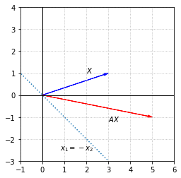
The effect of multiplication by \(A\) can be understood through its eigenvalues and eigenvectors. The first eigenvector of \(A\) lies in the direction of the line \(x_1=-x_2\). We label it \(V_1\) and observe that it gets scaled by a factor of 3 when multiplied by \(A\). The corresponding eigenvalue is \(\lambda_1 = 3\).
The other eigenvector, which we label \(V_2\), is orthogonal to the line \(x_1=-x_2\). This vector is left unchanged when multiplied by \(A\), which implies that \(\lambda_2 = 1\).
Since \(\{V_1, V_2\}\) form a basis for \(\mathbb{R}^2\), any other vector in \(\mathbb{R}^2\) can be written as a linear combination of these vectors. Let’s take the following vector \(X\) as an example.
To express \(X\) in terms of the eigenvectors, we have to solve the vector equation \(c_1V_1 + c_2V_2 = X\).
# Solve the matrix equation BC = X.  C is the vector of coefficients.
B = np.array([[1, 1],[-1,1]])
C = lag.SolveSystem(B,X)
print(C)
[[1.]
 [2.]]
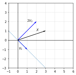
Let’s look at a visual representation of the linear combination \(X = V_1 + 2V_2\).
fig, ax = plt.subplots()

ax.arrow(0,0,3,1,fc='k',ec='k',**options)
ax.arrow(0,0,1,-1,fc='b',ec='b',**options)
ax.arrow(0,0,2,2,fc='b',ec='b',**options)
ax.plot(x,-x,ls=':')

ax.set_xlim(-1,6)
ax.set_ylim(-3,4)
ax.set_aspect('equal')
ax.set_xticks(np.arange(-1,7,step = 1))
ax.set_yticks(np.arange(-3,5,step = 1))

ax.text(1,2,'$2V_2$')
ax.text(2,1,'$X$')
ax.text(0.1,-1,'$V_2$')

ax.axvline(color='k',linewidth = 1)
ax.axhline(color='k',linewidth = 1)

ax.grid(True,ls=':')
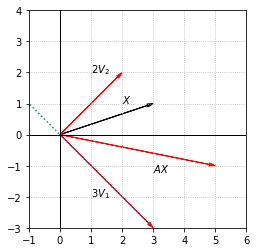
We can now understand, and compute, the product \(AX\) by evaluating the products of \(A\) with its eigenvectors.
fig, ax = plt.subplots()

ax.arrow(0,0,3,1,fc='k',ec='k',**options)
ax.arrow(0,0,3,-3,fc='r',ec='r',**options)
ax.arrow(0,0,2,2,fc='r',ec='r',**options)
ax.arrow(0,0,5,-1,fc='r',ec='r',**options)
ax.plot(x,-x,ls=':')

ax.set_xlim(-1,6)
ax.set_ylim(-3,4)
ax.set_aspect('equal')
ax.set_xticks(np.arange(-1,7,step = 1))
ax.set_yticks(np.arange(-3,5,step = 1))

ax.text(1,2,'$2V_2$')
ax.text(2,1,'$X$')
ax.text(3,-1.2,'$AX$')
ax.text(1,-2,'$3V_1$')

ax.axvline(color='k',linewidth = 1)
ax.axhline(color='k',linewidth = 1)

ax.grid(True,ls=':')
Computation of eigenvectors with SciPy
We now demonstrate how to compute eigenvalues and eigenvectors for any square matrix using the function \(\texttt{eig}\) from the SciPy \(\texttt{linalg}\) module. This function accepts an \(n\times n\) array representing a matrix and returns two arrays, one containing the eigenvalues, the other the eigenvectors. We examine the usage by supplying our projection matrix as the argument.
import scipy.linalg as sla

A = np.array([[0.2, -0.4],[-0.4, 0.8]])
print(A)
print('\n')

evalues,evectors = sla.eig(A)

print(evalues)
[[ 0.2 -0.4]
 [-0.4  0.8]]


[0.+0.j 1.+0.j]
The array of eigenvalues contains two entries that are in the format of \(\alpha + \beta j\), which represents a complex number. The symbol \(j\) is used for the imaginary unit. The value of \(\beta\) is zero for both of the eigenvalues, which means that they are both real numbers. The results confirm our conclusions that the eigenvalues are 0 and 1.
Next let’s look at the array of eigenvectors. We can slice the array into columns to give us convenient access to the vectors.
print(evectors)

V_1 = evectors[:,0:1]
V_2 = evectors[:,1:2]
[[-0.89442719  0.4472136 ]
 [-0.4472136  -0.89442719]]
We may not recognize the eigenvectors as those we found previously, but recall that eigenvectors are not unique. The \(\texttt{eig}\) function scales all the eigenvectors to unit length, and we arrive at the same result if we scale our choice of eigenvector.
V = np.array([[-2],[-1]])
print(V)
print('\n')
print(V/lag.Magnitude(V))
[[-2]
 [-1]]


[[-0.89442719]
 [-0.4472136 ]]
Example 2: Verifying eigenvectors using matrix multiplication
Let’s try another example with a \(3\times 3\) matrix.
B = np.array([[1,2, 0],[2,-1,4],[0,3,1]])
evalues, evectors = sla.eig(B)

print(evalues)
print('\n')
print(evectors)

V_1 = evectors[:,0:1]
V_2 = evectors[:,1:2]
V_3 = evectors[:,2:3]

E_1 = evalues[0]
E_2 = evalues[1]
E_3 = evalues[2]
[-4.12310563+0.j  1.        +0.j  4.12310563+0.j]


[[ 3.19250163e-01  8.94427191e-01  4.19279023e-01]
 [-8.17776152e-01 -1.03817864e-16  6.54726338e-01]
 [ 4.78875244e-01 -4.47213595e-01  6.28918535e-01]]
We don’t have the exact eigenvalues, but we can check that \(BV_i - \lambda_iV_i = 0\) for \(i=1, 2, 3\), allowing for the usual roundoff error.
print(B@V_1-E_1*V_1)
[[-4.44089210e-16+0.j]
 [ 2.22044605e-15+0.j]
 [-1.11022302e-15+0.j]]
Instead of \(BV_i - \lambda_iV_i = 0\) for each \(i\), we can package the calculations into a single matrix multiplication. If \(S\) is the matrix with columns \(V_i\), then \(BS\) is the matrix with columns \(BV_i\). This matrix should be compared to the matrix that has \(\lambda_iV_i\) as its columns. To construct this matrix we use a diagonal matrix \(D\), that has the \(\lambda_i\) as its diagonal entries. The matrix product \(SD\) will then have columns \(\lambda_iV_i\).
We can now simply check that \(BS-SD = 0\).
S = evectors

#  Since the eigenvalues are complex, it is best to use an array of complex numbers for D
D = np.zeros((3,3),dtype='complex128')
for i in range(3):
    D[i,i] = evalues[i]

print(D)
print('\n')
print(B@S-S@D)
[[-4.12310563+0.j  0.        +0.j  0.        +0.j]
 [ 0.        +0.j  1.        +0.j  0.        +0.j]
 [ 0.        +0.j  0.        +0.j  4.12310563+0.j]]


[[-4.44089210e-16+0.j -6.66133815e-16+0.j  4.44089210e-16+0.j]
 [ 2.22044605e-15+0.j  5.47907073e-16+0.j  0.00000000e+00+0.j]
 [-1.11022302e-15+0.j -1.11022302e-16+0.j  0.00000000e+00+0.j]]
Diagonal factorization
The calculation that we used to verify the eigenvalues and eigenvectors is also very useful to construct another important matrix factorization. Suppose that \(A\) is an \(n\times n\) matrix, \(D\) is a diagonal matrix with the eigenvalues of \(A\) along its diagonal, and \(S\) is the \(n\times n\) matrix with the eigenvectors of \(A\) as its columns. We have just seen that \(AS=SD\). If \(S\) is invertible, we may also write \(A=SDS^{-1}\), which is known as the diagonalization of \(A\).
The diagonalization of \(A\) is important because it provides us with a complete description of the action of \(A\) in terms of its eigenvectors. Consider an arbitrary vector \(X\), and the product \(AX\), computed by using the three factors in the diagonalization.
\(S^{-1}X\) computes the coordinates of \(X\) in terms of the eigenvectors of \(A\).
Multiplication by \(D\) then simply scales each coordinate by the corresponding eigenvalue.
Multiplication by \(S\) gives the results with respect to the standard basis.
This understanding does not provide a more efficient way of computing the product \(AX\), but it does provide a much more general way of understanding the result of a matrix-vector multiplication. As we will see in the next section, the diagonalization also provides a significant shortcut in computing powers of \(A\).
It should be noted that diagonalization of an \(n\times n\) matrix \(A\) is not possible when the eigenvectors of \(A\) form a linearly dependent set. In that case the eigenvectors do not span \(\mathbb{R}^n\), which means that not every \(X\) in \(\mathbb{R}^n\) can be written as a linear combination of the eigenvectors. In terms of the computation above, \(S\) will not be invertible exactly in this case.
Exercises
Exercise 1: Find the diagonalization of the matrix from Example 1.
A = np.array([[2, -1],[-1, 2]])

## Code solution here
Exercise 2: Find the diagonalization of the following matrix.
## Code solution here.
Exercise 3: Write a function that accepts an \(n\times n\) matrix \(A\) as an argument, and returns the three matrices \(S\), \(D\), and \(S^{-1}\) such that \(A=SDS^{-1}\). Make use of the \(\texttt{eig}\) function in SciPy.
## Code solution here.
Exercise 4: Construct a \(3\times 3\) matrix that is not diagonal and has eigenvalues 2, 4, and 10.
## Code solution here.
Exercise 5: Suppose that \(C = QDQ^{-1}\) where
\((a)\) Give a basis for \(\mathcal{N}(C)\)
\((b)\) Find all the solutions to \(CX = V + W\)
## Code solutions here.