Linear Systems
import laguide as lag
import numpy as np
import scipy.linalg as sla
%matplotlib inline
import matplotlib.pyplot as plt
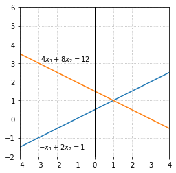
Exercise 1: Consider the system of equations given below. Find a value for the coefficient \(a\) so that the system has exactly one solution. For that value of \(a\), find the solution to the system of equations and plot the lines formed by your equations to check your answer.
If \(a=1\) the two lines are parallel and do not intersect. For any other value of \(a\) the lines intersect at exactly one point. For example, we take \(a = -1\). By plotting the two lines formed by these equations and examining where they intersect we can see that the solution to this system is \(x_1 = 1,\) \(x_2 = 1\)
x=np.linspace(-5,5,100)

fig, ax = plt.subplots()
ax.plot(x,(x+1)/2)
ax.plot(x,(12-4*x)/8)

ax.text(-2.9,3.1,'$4x_1 + 8x_2 = 12$')
ax.text(-3,-1.6,'$-x_1 + 2x_2 = 1$')

ax.set_xlim(-4,4)
ax.set_ylim(-2,6)
ax.axvline(color='k',linewidth = 1)
ax.axhline(color='k',linewidth = 1)

ax.set_xticks(np.linspace(-4,4,9))
ax.set_yticks(np.linspace(-2,6,9))
ax.set_aspect('equal')
ax.grid(True,ls=':')
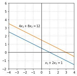
Exercise 2: Find a value for the coefficient \(a\) so that the system has no solution. Plot the lines formed by your equations to verify there is no solution.
If \(a = 1\) then the lines are parallel and there is no solution to the system.
x=np.linspace(-5,5,100)

fig, ax = plt.subplots()
ax.plot(x,(1-x)/2)
ax.plot(x,(12-4*x)/8)

ax.text(-2.8,3.1,'$4x_1 + 8x_2 = 12$')
ax.text(0.4,-1.4,'$x_1 + 2x_2 = 1$')

ax.set_xlim(-4,4)
ax.set_ylim(-2,6)
ax.axvline(color='k',linewidth = 1)
ax.axhline(color='k',linewidth = 1)

ax.set_xticks(np.linspace(-4,4,9))
ax.set_yticks(np.linspace(-2,6,9))
ax.set_aspect('equal')
ax.grid(True,ls=':')
Exercise 3: Consider the system of equations given below. Under what conditions on the coefficients \(a,b,c,d,e,f\) does this system have only one solution? No solutions? An infinite number of solutions? (Think about what must be true of the slopes and intercepts of the lines in each case.)
Using algebra, we can convert the arbitrary equation \(ax_1 + bx_2 = c\) to its slope-intercept form \(x_2 = - \frac{a}{b}x_1 + \frac{c}{b}\). Two lines intersect only once in the plane if and only if their slopes are different. Therefore if \(\frac{a}{b} \neq \frac{d}{e}\) then the system has exactly one solution. In the case that the slopes are equal, we examine the y-intercepts of the equations to determine whether there exists no solutions or an infinite number of solutions. If \(\frac{c}{b} = \frac{f}{e}\) then the y-intercepts are equal and the two equations describe the same line. In this case there are an infinite number of solutions. On the other hand, if \(\frac{c}{b} \neq \frac{f}{e}\) then the lines are parallel and there exists no solutions. In summary:
If \(\frac{a}{b} \neq \frac{d}{e}\) then there exists exactly one solution
If \(\frac{a}{b} = \frac{d}{e}\) and \(\frac{c}{b} = \frac{f}{e}\) then there are an infinite number of solutions
If \(\frac{a}{b} = \frac{d}{e}\) and \(\frac{c}{b} \neq \frac{f}{e}\) then there are no solutions
Gaussian Elimination
Exercise 1: In the system below, use a row operation functions to produce a zero coefficient in the location of the coefficient 12. Do this first by hand and then create a NumPy array to represent the system and use the row operation functions. (There are two ways to create the zero using \(\texttt{RowAdd}\). Try to find both.)
C = np.array([[4,-2,7,2],[1,3,12,4],[-7,0,-3,-1]])
C1 = lag.RowAdd(C,0,1,-12/7)
C2 = lag.RowAdd(C,2,1,4)
print(C,'\n')
print(C1,'\n')
print(C2,'\n')
[[ 4 -2  7  2]
 [ 1  3 12  4]
 [-7  0 -3 -1]]

[[ 4.         -2.          7.          2.        ]
 [-5.85714286  6.42857143  0.          0.57142857]
 [-7.          0.         -3.         -1.        ]]

[[  4.  -2.   7.   2.]
 [-27.   3.   0.   0.]
 [ -7.   0.  -3.  -1.]]
Exercise 2: Create a NumPy array to represent the system below. Determine which coefficient should be zero in order for the system to be upper triangular. Use \(\texttt{RowAdd}\) to carry out the row operation and then print your results.
A = np.array([[3,4,-1,-6],[0,-2,10,-8],[0,4,-2,-2]])

# B is obtained after performing RowAdd on A.
B = lag.RowAdd(A, 1, 2, 2)
print(B)
[[  3.   4.  -1.  -6.]
 [  0.  -2.  10.  -8.]
 [  0.   0.  18. -18.]]
Exercise 3: Carry out the elimination process on the following system. Define a NumPy array and make use of the row operation functions. Print the results of each step. Write down the upper triangular system represented by the array after all steps are completed.
A = np.array([[1,-1,1,3],[2,1,8,18],[4,2,-3,-2]])
A1 = lag.RowScale(A,0,1.0/A[0][0])
A2 = lag.RowAdd(A1,0,1,-A[1][0])
A3 = lag.RowAdd(A2,0,2,-A2[2][0])
A4 = lag.RowScale(A3,1,1.0/A3[1][1])
A5 = lag.RowAdd(A4,1,2,-A4[2][1])
A6 = lag.RowScale(A5,2,1.0/A5[2][2])
print(A,'\n')
print(A1,'\n')
print(A2,'\n')
print(A3,'\n')
print(A4,'\n')
print(A5,'\n')
print(A6,'\n')
[[ 1 -1  1  3]
 [ 2  1  8 18]
 [ 4  2 -3 -2]]

[[ 1. -1.  1.  3.]
 [ 2.  1.  8. 18.]
 [ 4.  2. -3. -2.]]

[[ 1. -1.  1.  3.]
 [ 0.  3.  6. 12.]
 [ 4.  2. -3. -2.]]

[[  1.  -1.   1.   3.]
 [  0.   3.   6.  12.]
 [  0.   6.  -7. -14.]]

[[  1.  -1.   1.   3.]
 [  0.   1.   2.   4.]
 [  0.   6.  -7. -14.]]

[[  1.  -1.   1.   3.]
 [  0.   1.   2.   4.]
 [  0.   0. -19. -38.]]

[[ 1. -1.  1.  3.]
 [ 0.  1.  2.  4.]
 [-0. -0.  1.  2.]]
Exercise 4: Use row operations on the system below to produce an lower triangular system. The first equation of the lower triangular system should contain only \(x_1\) and the second equation should contain only \(x_1\) and \(x_2\).
A = np.array([[1,2,1,3],[3,-1,-3,-1],[2,3,1,4]])
print("A: \n", A, '\n')

B = lag.RowAdd(A, 2, 0, -1)
C = lag.RowAdd(B, 2, 1, 3)
L = lag.RowAdd(C, 1, 0, 1/8)

print("L: \n", L, '\n')
A:
 [[ 1  2  1  3]
 [ 3 -1 -3 -1]
 [ 2  3  1  4]]

L:
 [[ 0.125  0.     0.     0.375]
 [ 9.     8.     0.    11.   ]
 [ 2.     3.     1.     4.   ]]
The corresponding lower triangular system is
Exercise 5: Use elimination to determine whether the following system is consistent or inconsistent.
# A is the array of numbers corresponding to the given system.
A = np.array([[1,-1,-1,4],[2,-2,-2,8],[5,-5,-5,20]])

# B1 and B2 are obtained by performing row operations on A.
B1 = lag.RowAdd(A, 0, 1, -2)
B2 = lag.RowAdd(B1, 0, 2, -5)

print(B1)
print(B2)
[[ 1. -1. -1.  4.]
 [ 0.  0.  0.  0.]
 [ 5. -5. -5. 20.]]
[[ 1. -1. -1.  4.]
 [ 0.  0.  0.  0.]
 [ 0.  0.  0.  0.]]
In this system the second equation and third equation are just multiples of the first. Any solution to one of the equations is a solution to all three equations. We can get a solution to the first equation by choosing values for \(x_2\) and \(x_3\) and then calculating the value of \(x_1\) that satisfies the equation. One such solution is \(x_1 = 6\), \(x_2=1\), \(x_3=1\).
Exercise 6: Use elimination to show that this system of equations has no solution.
# A is the array of numbers corresponding to the given system of equations.
A = np.array([[1,1,1,0],[1,-1,3,3],[-1,-1,-1,2]])

B1 = lag.RowAdd(A, 0, 1, -1)
print(B1)

B2 = lag.RowAdd(B1, 0, 2, 1)
print(B2)
[[ 1.  1.  1.  0.]
 [ 0. -2.  2.  3.]
 [-1. -1. -1.  2.]]
[[ 1.  1.  1.  0.]
 [ 0. -2.  2.  3.]
 [ 0.  0.  0.  2.]]
The third row of \(\texttt{B2}\) indicates that the system is inconsistent. This row represents the equation \(0x_3 = 2\), which cannot be true for any value of \(x_3\).
Exercise 7: Use \(\texttt{random}\) module to produce a \(3\times 4\) array which contains random integers between \(0\) and \(5\). Write code that performs a row operation that produces a zero in the first row, third column. Run the code several times to be sure that it works on different random arrays. Will the code ever fail?
## Code solution here.

A = np.random.randint(0,5, size = (3,4))

print("A: \n", A, '\n')

if A[1,2] == 0:
    A = lag.RowSwap(A, 0, 1)
else:
    A = lag.RowAdd(A, 1, 0, -A[0,2]/A[1,2])

print("A after one row operation: \n", A, '\n')
A:
 [[0 4 3 4]
 [2 1 2 2]
 [4 4 3 3]]

A after one row operation:
 [[-3.   2.5  0.   1. ]
 [ 2.   1.   2.   2. ]
 [ 4.   4.   3.   3. ]]
The code will not fail to produce a matrix with a zero in the specified position.
Exercise 8: Starting from the array that represents the upper triangular system in Example 1 (\(\texttt{A5}\)), use the row operations to produce an array of the following form. Do one step at a time and again print your results to check that you are successful.
B = np.array([[1,-1,1,3],[0,1,2,4],[0,0,1,2]])
B1 = lag.RowAdd(B,1,0,1)
B2 = lag.RowAdd(B1,2,0,-3)
B3 = lag.RowAdd(B2,2,1,-2)
print(B,'\n')
print(B1,'\n')
print(B2,'\n')
print(B3,'\n')
[[ 1 -1  1  3]
 [ 0  1  2  4]
 [ 0  0  1  2]]

[[1. 0. 3. 7.]
 [0. 1. 2. 4.]
 [0. 0. 1. 2.]]

[[1. 0. 0. 1.]
 [0. 1. 2. 4.]
 [0. 0. 1. 2.]]

[[1. 0. 0. 1.]
 [0. 1. 0. 0.]
 [0. 0. 1. 2.]]
Exercise 9: Redo Example 2 using the \(\texttt{random}\) module to produce a \(3\times 4\) array made up of random floats instead of random integers.
D = np.random.rand(3,4)
D1 = lag.RowScale(D,0,1.0/D[0][0])
D2 = lag.RowAdd(D1,0,1,-D[1][0])
D3 = lag.RowAdd(D2,0,2,-D2[2][0])
D4 = lag.RowScale(D3,1,1.0/D3[1][1])
D5 = lag.RowAdd(D4,1,2,-D4[2][1])
D6 = lag.RowScale(D5,2,1.0/D5[2][2])
print(D,'\n')
print(D1,'\n')
print(D2,'\n')
print(D3,'\n')
print(D4,'\n')
print(D5,'\n')
print(D6,'\n')
[[0.90838555 0.79006406 0.98618885 0.90765811]
 [0.60957668 0.83222735 0.48921852 0.49499601]
 [0.40006273 0.21571988 0.69192963 0.13688866]]

[[1.         0.86974529 1.08565009 0.9991992 ]
 [0.60957668 0.83222735 0.48921852 0.49499601]
 [0.40006273 0.21571988 0.69192963 0.13688866]]

[[ 1.00000000e+00  8.69745293e-01  1.08565009e+00  9.99199197e-01]
 [ 1.11022302e-16  3.02050904e-01 -1.72568455e-01 -1.14092522e-01]
 [ 4.00062729e-01  2.15719877e-01  6.91929625e-01  1.36888659e-01]]

[[ 1.00000000e+00  8.69745293e-01  1.08565009e+00  9.99199197e-01]
 [ 1.11022302e-16  3.02050904e-01 -1.72568455e-01 -1.14092522e-01]
 [ 5.55111512e-17 -1.32232799e-01  2.57601488e-01 -2.62853698e-01]]

[[ 1.00000000e+00  8.69745293e-01  1.08565009e+00  9.99199197e-01]
 [ 3.67561564e-16  1.00000000e+00 -5.71322425e-01 -3.77726141e-01]
 [ 5.55111512e-17 -1.32232799e-01  2.57601488e-01 -2.62853698e-01]]

[[ 1.00000000e+00  8.69745293e-01  1.08565009e+00  9.99199197e-01]
 [ 3.67561564e-16  1.00000000e+00 -5.71322425e-01 -3.77726141e-01]
 [ 1.04114846e-16  0.00000000e+00  1.82053924e-01 -3.12801483e-01]]

[[ 1.00000000e+00  8.69745293e-01  1.08565009e+00  9.99199197e-01]
 [ 3.67561564e-16  1.00000000e+00 -5.71322425e-01 -3.77726141e-01]
 [ 5.71890147e-16  0.00000000e+00  1.00000000e+00 -1.71818039e+00]]
Exercise 10: Write a loop that will execute the elimination code in Example 2 on 1000 different \(3\times 4\) arrays of random floats to see how frequently it fails.
for count in range(1000):
    E = np.random.rand(3,4)
    E1 = lag.RowScale(E,0,1.0/E[0][0])
    E2 = lag.RowAdd(E1,0,1,-E[1][0])
    E3 = lag.RowAdd(E2,0,2,-E2[2][0])
    E4 = lag.RowScale(E3,1,1.0/E3[1][1])
    E5 = lag.RowAdd(E4,1,2,-E4[2][1])
    E6 = lag.RowScale(E5,2,1.0/E5[2][2])
Matrix Algebra
Exercise 1: Calculate \(-2E\), \(G+F\), \(4F-G\), \(HG\), and \(GE\) using the following matrix definitions. Do the exercise on paper first, then check by doing the calculation with NumPy arrays.
E = np.array([[5],[-2]])
F = np.array([[1,6],[2,0],[-1,-1]])
G = np.array([[2,0],[-1,3],[-1,6]])
H = np.array([[3,0,1],[1,-2,2],[3,4,-1]])
print(-2*E,'\n')
print(G+F,'\n')
print(4*F-G,'\n')
print(H@G,'\n')
print(G@E)
[[-10]
 [  4]]
[[ 3  6]
 [ 1  3]
 [-2  5]]

[[  2  24]
 [  9  -3]
 [ -3 -10]]

[[5 6]
 [2 6]
 [3 6]]

[[ 10]
 [-11]
 [-17]]
Exercise 2: Find the values of \(x\) and \(y\) so that this equation holds.
Recall that matrix multiplication can be carried out column by column. Given a matrix equation of the form \(AB = C\), multiplying \(A\) by the \(j^{\text{th}}\) column of \(B\) gives the \(j^{\text{th}}\) column of \(C\). This view of matrix multiplication gives the following linear system which we can solve with elimination
A = np.array([[1,3,10],[-4,2,16]])
A1 = lag.RowAdd(A,0,1,4)
A2 = lag.RowScale(A1,1,1/14)
A3 = lag.RowAdd(A2,1,0,-3)
print(A,'\n')
print(A1,'\n')
print(A2,'\n')
print(A3)
[[ 1  3 10]
 [-4  2 16]]

[[ 1.  3. 10.]
 [ 0. 14. 56.]]

[[ 1.  3. 10.]
 [ 0.  1.  4.]]

[[ 1.  0. -2.]
 [ 0.  1.  4.]]
Therefore \(x = -2\) and \(y = 4\).
Alternatively, if we carry out the matrix multiplication completely, we arrive at the same system to be solved.
Exercise 3: Define NumPy arrays for the matrices \(H\) and \(G\) given below.
\((a)\) Multiply the second and third column of \(H\) with the first and second row of \(G\). Use slicing to make subarrays. Does the result have any relationship to the full product \(HG\)?
\((b)\) Multiply the first and second row of \(H\) with the second and third column of \(G\). Does this result have any relationship to the full product \(HG\)?
H = np.array([[3,3,-1],[-3,0,8],[1,6,5]])
G = np.array([[1,5,2,-3],[7,-2,-3,0],[2,2,4,6]])

print(H@G,'\n')
print(H[:,1:3]@G[0:2,:],'\n')
print(H[0:2,:]@G[:,1:3])
[[ 22   7  -7 -15]
 [ 13   1  26  57]
 [ 53   3   4  27]]

[[ -4  17   9  -9]
 [ 56 -16 -24   0]
 [ 41  20  -3 -18]]

[[ 7 -7]
 [ 1 26]]
The second product is a \(2 \times 2\) matrix that is a submatrix of the larger matrix \(HG\).
Exercise 4: Generate a \(4\times 4\) matrix \(B\) with random integer entries. Compute matrices \(P = \frac12(B+B^T)\) and \(Q = \frac12(B-B^T)\). Rerun your code several times to get different matrices. What do you notice about \(P\) and \(Q\)? Explain why it must always be true.
B = np.random.randint(size=(4,4),high=10,low=-10)
P = 1/2*(B+B.transpose())
Q = 1/2*(B-B.transpose())
print(B,'\n')
print(P,'\n')
print(Q)
[[  5  -7   4   2]
 [  9  -3   2   8]
 [ -2   7  -5   3]
 [  0 -10   7   2]]

[[ 5.   1.   1.   1. ]
 [ 1.  -3.   4.5 -1. ]
 [ 1.   4.5 -5.   5. ]
 [ 1.  -1.   5.   2. ]]

[[ 0.  -8.   3.   1. ]
 [ 8.   0.  -2.5  9. ]
 [-3.   2.5  0.  -2. ]
 [-1.  -9.   2.   0. ]]
\(P\) is always a symmetric matrix and \(Q\) is always a skew-symmetric matrix.
To see why \(P\) is always symmetric, recall that \(P\) being symmetric is equivalent to saying \(p_{ij} = p_{ji}\) for all entries \(p_{ij}\) in \(P\). Now notice that
and therefore \(P\) is symmetric.
To see why \(Q\) is always skew-symmetric, recall that \(Q\) being skew-symmetric is equivalent to saying \(q_{ij} = -q_{ji}\) for all entries \(q_{ij}\) in \(Q\). Now notice that
and therefore \(Q\) is skew-symmetric.
Exercise 5: Just as the elements of a matrix can be either integers or real numbers, we can also have a matrix with elements that are themselves matrices. A block matrix is any matrix that we have interpreted as being partitioned into these submatrices. Evaluate the product \(HG\) treating the \(H_i\)’s and \(G_j\)’s as the elements of their respective matrices. If we have two matrices that can be multiplied together normally, does any partition allow us to multiply using the submatrices as the elements?
H = np.array([[1,3,2,0],[-1,0,3,3],[2,2,-2,1],[0,1,1,4]])
G = np.array([[3,0,5],[1,1,-3],[2,0,1],[0,2,1]])b
H1 = np.array([[1,3],[-1,0]])
H2 = np.array([[2,0],[3,3]])
H3 = np.array([[2,2],[0,1]])
H4 = np.array([[-2,1],[1,4]])
G1 = np.array([[3,0],[1,1]])
G2 = np.array([[5],[-3]])
G3 = np.array([[2,0],[0,2]])
G4 = np.array([[1],[1]])
HG1 = H1@G1 + H2@G3
HG2 = H1@G2 + H2@G4
HG3 = H3@G1 + H4@G3
HG4 = H3@G2 + H4@G4
print(H@G,'\n')
print(HG1,'\n')
print(HG2,'\n')
print(HG3,'\n')
print(HG4)
  File "<ipython-input-18-7b2e27f83d3b>", line 2
    G = np.array([[3,0,5],[1,1,-3],[2,0,1],[0,2,1]])b
                                                    ^
SyntaxError: invalid syntax
Not every partition of a matrix will let us multiply them in this way. If we had instead partitioned \(H\) like this:
then many of the products calculated above (such as \(H_1G_1\)) would not be defined.
Inverse Matrices
Exercise 1: Solve the following system of equations using an inverse matrix.
We can write the matrix equation \(AX = B\) for the given system of equation which looks like:
A = np.array([[2,3,1],[3,3,1],[2,4,1]])

print("A: \n", A, '\n')

A_inv = lag.Inverse(A)
b = np.array([[4],[8],[5]])

print("b: \n", b, '\n')
print("A_inv: \n", A_inv, '\n')
x = A_inv@b

print("x: \n", x, '\n')
Exercise 2: Let \(A\) and \(B\) be two random \(4\times 4\) matrices. Demonstrate using Python that \((AB)^{-1}=B^{-1}A^{-1}\) for the matrices.
## Code solution here
Exercise 3: Explain why \((AB)^{-1}=B^{-1}A^{-1}\) by using the definition given in this section.
Exercise 4: Solve the system \(AX=B\) by finding \(A^{-1}\) and computing \(X=A^{-1}B\).
A = np.array([[1,2,-3],[-1,1,-1],[0,-2,3]])
print("A: \n", A, '\n')

A_inverse = lag.Inverse(A)
B = np.array([[1],[1],[1]])

print("A inverse is : \n", A_inverse, '\n')

X = A_inverse@B

print("X: \n", X, '\n')
Exercise 5: Find a \(3 \times 3 \) matrix \(Y\) such that \(AY = C\).
A = np.array([[3,1,0],[5,2,1],[0,2,3]])
C = np.array([[1,2,1],[3,4,0],[1,0,2]])

print("A: \n", A, '\n')
print("C: \n", C, '\n')

A_inv = lag.Inverse(A)
Y = A_inv@C

print("A inverse is : \n", A_inv, '\n')
print("Y: \n", Y, '\n')
Exercise 6: Let \(A\) be a random \(4 \times 1\) matrix and \(B\) is a random \( 1 \times 4 \) matrix. Use Python to demonstrate that the product \( AB \) is not invertible. Do you expect this to be true for any two matrices \(P\) and \(Q\) such that \(P\) is an \( n \times 1 \) matrix and \(Q\) is a \( 1 \times n\) matrix ? Explain.
A = np.random.randint(0,9, size = (4,1))
B = np.random.randint(0,9, size = (1,4))

print("A: \n", A, '\n')
print("B: \n", B, '\n')

AB = A@B
AB = lag.FullRowReduction(AB)

print("AB: \n", AB, '\n')
A:
 [[7]
 [0]
 [2]
 [7]]

B:
 [[6 7 7 5]]

AB:
 [[1.         1.16666667 1.16666667 0.83333333]
 [0.         0.         0.         0.        ]
 [0.         0.         0.         0.        ]
 [0.         0.         0.         0.        ]]
It can be clearly seen from the above code cell that the reduced form of the product \(AB\) contains zero enteries on the diagonal. This shows that \(AB\) is not invertible. It is expected to be true for any two general matrices \(P\) and \(Q\) where \(P\) is an \( n \times 1 \) matrix and \(Q\) is a \( 1 \times n\) matrix.
Let $\( P = \left[ \begin{array}{rrrr} a \\ b \\ c \\ d\\..\\.. \end{array}\right] \)\( and \)\( Q = \left[ \begin{array}{rrrr} w & x &y&z&.&.&. \end{array}\right] \)$
If we perform a \(\texttt{RowAdd}\) to create a zero at any position in a row using another row, the entire row becomes zero. Notice that each row is just a multiple of the first row. This means that when we carry out row reduction on \(PQ\), the resulting upper triangular matrix have zeros in all entries except for the first row. This implies that the product \(PQ\) is non-invertible.
Exercise 7: Let \(A\) be a random \( 3 \times 3\) matrices. Demonstrate using Python that \((A^T)^{-1} = (A^{-1})^T\) for the matrix. Use this property to explain why \(A^{-1}\) must be symmetric if \(A\) is symmetric.
A = np.random.randint(0,9, size = (3,3))

print("A: \n", A, '\n')

# Create the inverse of A and its transpose
A_inv = lag.Inverse(A)
A_inv_trans = A_inv.transpose()

print("A_inv_transpose: \n", np.round(A_inv_trans,8), '\n')

# Create the transpose of A and its inverse
A_trans = A.transpose()
A_trans_inv = lag.Inverse(A_trans)

print("A_trans_inverse: \n", np.round(A_trans_inv,8), '\n')

# checking if the transpose of A inverse and the inverse of A transpose are equal.
if (np.array_equal(A_trans_inv, A_inv_trans)):
    print("A_inverse_transpose and A_transpose_inverse are equal. ")
else:
    print("A_inverse_transpose and A_transpose_inverse are not equal. ")
A:
 [[3 0 1]
 [2 6 3]
 [4 5 8]]

A_inv_transpose:
 [[ 0.38823529 -0.04705882 -0.16470588]
 [ 0.05882353  0.23529412 -0.17647059]
 [-0.07058824 -0.08235294  0.21176471]]

A_trans_inverse:
 [[ 0.38823529 -0.04705882 -0.16470588]
 [ 0.05882353  0.23529412 -0.17647059]
 [-0.07058824 -0.08235294  0.21176471]]

A_inverse_transpose and A_transpose_inverse are not equal.
From the computations done in the code cell above, we verified that \( (A^{-1})^T = (A^T)^{-1} \). If \(A\) is symmetric, then \(A^T = A\) and we can replace \(A^T\) with \(A\) on the right side of the equation to get \((A^{-1})^T = A^{-1} \), which means that \(A^{-1}\) is also symmetric.
Exercise 8: Consider the following \( 4 \times 4 \) matrix:
\((a)\) Find the condition on \(x_1\), \(x_2\), \(x_3\) or \(x_4\) for which \(A^{-1}\) exists. Assuming that condition is true, find the inverse of \(A\).
\((b)\) Use Python to check if \( A^{-1}A = I \) when \(x_1 = 4\), \(x_2 = 1\), \(x_3 = 1\), and \(x_4 = 3\).
Solution:
(a) After carrying out row operations on \(A\), we get the following upper triangular matrix.
\(A\) will be invertible if and only if all the diagonal enteries are non-zero, so \(A\) will be invertible if and only if \(x_2\neq 0\). In this case, \([A|I]\) is
row operations give \(A^{-1}\) as follows.
## Part (b)

x_1 = 1
x_2 = 2
x_3 = 4
x_4 = 0

A = np.array([[4,x_1,0,0],[0,x_2,0,0],[0,x_3,1,0],[0,x_4,0,3]])
A_inv = np.array([[1/4,-x_1/4/x_2,0,0],[0,x_2,0,0],[0,-x_3/x_2,1,0],[0,-x_4/3/x_2,0,1/3]])

print("A@A_inv: \n", A@A_inv,'\n')
A@A_inv:
 [[1.  1.5 0.  0. ]
 [0.  4.  0.  0. ]
 [0.  6.  1.  0. ]
 [0.  0.  0.  1. ]]
## Code solution here
Exercise 9: Apply the methods used in this section to compute a right inverse of the matrix \(A\).
Let \(C\) be the right inverse of \(A\), then \(AC= I\), and \(C\) is a \( 4 \times 2 \) matrix.
If we understand the product \(AC\) in terms of the columns of \(C\), we get two linear systems to solve for \(x_i\) and \(y_i\) which are as follows:
It can be clearly seen that \(x_3, x_4, y_3\), and \(y_4\) are free variables due to which there are infinite number of matrices \(C\) which can be the right inverse of \(A\). In other words, \(C\) is not unique. One possibility is:
We check that \( AC = I \) in the code cell below.
A = np.array([[1,0,0,2],[0,-1,1,4]])
C = np.array([[1,0],[0,-1],[0,0],[0,0]])

print("AC = \n", A@C, '\n')
LU Factorization
Exercise 1: Solve \( AX = B \) using \( A = LU \) and the \(L\), \(U\), and \(B\) given below. Compute \(LUX\) to verify your answer.
## Code solution here.
Exercise 2: Solve \( AX = B \) using \( A = LU \) and the \(L\), \(U\), and \(B\) given below. Compute \(LUX\) to verify your answer.
## Code solution here.
Exercise 3: Write a function called \(\texttt{ForwardSubstitution}\) that will solve a lower triangular system \(LY=B\). It will be helpful to go back and look at the code for \(\texttt{BackSubstitution}\).
## Code solution here.
Exercise 4: Let \(A\), \(B\), and \(C\) be the following matrices:
\((a)\) Find an elementary matrix \(E\) such that \(EA = B\). Verify with a computation.
\((b)\) Find an elementary matrix \(F\) such that \( FB = C\). Verify with a computation.
# Building the matrix A
A = np.array([[1,2,4],[2,1,3],[1,0,2]])
I = np.eye(3)
print("A: \n", A, '\n')

# Part (a)
B = lag.RowAdd(A, 0, 2, 1)
E = lag.RowAdd(I, 0, 2, 1)

print("B: \n", B, '\n')
print("E: \n", E, '\n')
print("EA: \n", E@A, '\n')

# Part (b)
# Building the matrix B
B = np.array([[1,2,4],[2,1,3],[2,2,6]])

C = lag.RowAdd(B, 2, 1, -1)
F = lag.RowAdd(I, 2, 1, -1)

print("C: \n", C, '\n')
print("F: \n", F, '\n')

print("FB: \n", F@B, '\n')
Exercise 5: Consider the following \(3\times 3\) matrix :
\((a)\) Find elementary matrices \(E_1\), \(E_2\), and \(E_3\) such that \( E_3E_2E_1A = U \) where \(U\) is an upper triangular matrix.
\((b)\) Find \(L\) using the inverses of \(E_1\), \(E_2\), \(E_3\), and verify that \( A = LU \).
# Create the matrix A
A = np.array([[2,1,1],[6,4,5],[4,1,3]])
I = np.eye(3)
print("A: \n", A, '\n')

#Part (a):
B1 = lag.RowAdd(A, 0, 1, -3)
E1 = lag.RowAdd(I, 0, 1, -3)

B2 = lag.RowAdd(B1, 0, 2, -2)
E2 = lag.RowAdd(I, 0, 2, -2)

U = lag.RowAdd(B2, 1, 2, 1)
E3 = lag.RowAdd(I, 1, 2, 1)


print("E1: \n", E1, '\n')
print("E2: \n",E2, '\n')
print("E3: \n", E3, '\n')
print("U: \n", U, '\n')

# Part (b)
L1 = sla.inv(E1)
L2 = sla.inv(E2)
L3 = sla.inv(E3)

L = L1@L2@L3

print("L: \n", L, '\n' )
print("LU: \n", L@U, '\n')
Exercise 6: Compute the \(LDU\) factorization of the following matrix and verify that \(A = LDU\).
# Create the matrix A
A = np.array([[1,1,1],[3,5,6],[-2,2,7]])
I = np.eye(3)
print("A: \n", A, '\n')

B1 = lag.RowAdd(A, 0, 1, -3)
E1 = lag.RowAdd(I, 0, 1, -3)

B2 = lag.RowAdd(B1, 0, 2, 2)
E2 = lag.RowAdd(I, 0, 2, 2)

B3 = lag.RowAdd(B2, 1, 2, -2)
E3 = lag.RowAdd(I, 1, 2, -2)

print("B3: \n", B3, '\n')

L1 = sla.inv(E1)
L2 = sla.inv(E2)
L3 = sla.inv(E3)

# creating lower triangular matrix L
L = L1@L2@L3

# creating row echelon form of A
U1 = lag.RowScale(B3, 1, 1/2)
U = lag.RowScale(U1, 2, 1/3)

# creating diagonal matrix D
D = np.array([[1,0,0],[0,2,0],[0,0,3]])

print("L: \n", L, '\n')
print("U: \n", U, '\n')
print("D: \n", D, '\n')

print("LDU: \n", L@D@U, '\n' )
Exercise 7: Find \(P, L,\) and \(U\) such that \(PA = LU\). Following the discussion in this section, \(P\) should be a permutation matrix, \(L\) should be a lower triangular matrix with ones long the main diagonal, and \(U\) should be an upper triangular matrix.
# Building the matrix A
A = np.array([[1,3,2],[-2,-6,1],[2,5,7]])
I = np.eye(3)

B1 = lag.RowAdd(A, 0, 1, 2)
E1 = lag.RowAdd(I, 0, 1, 2)

B2 = lag.RowAdd(B1, 0, 2, -2)
E2 = lag.RowAdd(I, 0, 2, -2)

print("B1: \n", B1, '\n')
print("B2: \n", B2, '\n')

# Since we cannot perform futher row reduction in this form, we need to swap the second and third rows.

# P is the permutation matrix

P = lag.RowSwap(I, 1, 2)

print("P: \n", P, '\n')
print("PA: \n", P@A, '\n')

B = lag.RowAdd(P@A, 0, 1, -2)
F1 = lag.RowAdd(I, 0, 1, -2)

print("B: \n", B, '\n')

# U is the upper triangular matrix
U = lag.RowAdd(B, 0, 2, 2)
F2 = lag.RowAdd(I, 0, 2, 2)

print("U: \n", U, '\n')

L1 = sla.inv(F1)
L2 = sla.inv(F2)

L = L1@L2

print("L: \n", L, '\n')

print("LU: \n", L@U, '\n')

# From here, we can see that PA = LU.
Exercise 8: Use SciPy to compute the \(PLU\) factorization of a \(3\times 3\) matrix. Replicate the results using the row operations functions in \(\texttt{laguide}\).
## Code Solution here
Applications
Interpolation
Exercise 1: In 2017, researchers from the Universities of British Columbia, Alberta, and Toronto published their findings regarding the population of snowshoe hares around Kluane Lake, Yukon. They measured the density of hares per hectare, taking a reading once every two years. Here are some of their measurements:
Measurement # |
Density per ha. |
|---|---|
1 |
0.26 |
2 |
0.20 |
3 |
1.17 |
4 |
2.65 |
5 |
0.14 |
6 |
0.42 |
7 |
1.65 |
8 |
2.73 |
9 |
0.09 |
10 |
0.21 |
\((a)\) Find the unique ninth degree polynomial whose graph passes through each of these points. Plot the data points together with the graph of the polynomial to observe the fit.
\((b)\) Using the polynomial that we found, what should we expect the density of hares to be if we measured their population in the year between the third and fourth measurement? What about between the fourth and the fifth?
\((c)\) Why might this method of interpolation not be an appropriate model of our data over time?
x = np.array([1,2,3,4,5,6,7,8,9,10])
y = np.array([0.26,0.2,1.17,2.65,0.14,0.42,1.65,2.73,0.09,0.21])

A = np.zeros((10,10),dtype=int)
B = np.zeros((10,1))

for i in range(10):
    B[i,0] = y[i]
    for j in range(10):
        A[i,j] = x[i]**(j)

coeffs = lag.SolveSystem(A,B)

x_fit = np.linspace(x[0],x[9],100)
y_fit = coeffs[0] + coeffs[1]*x_fit + coeffs[2]*x_fit**2 + coeffs[3]*x_fit**3 + coeffs[4]*x_fit**4 + coeffs[5]*x_fit**5 + coeffs[6]*x_fit**6 + coeffs[7]*x_fit**7 + coeffs[8]*x_fit**8 + coeffs[9]*x_fit**9

fig,ax = plt.subplots()

ax.scatter(x,y,color='red');
ax.plot(x_fit,y_fit,'b');
ax.set_xlim(0,11);
ax.set_ylim(-7,7);
ax.set_xlabel('x');
ax.set_ylabel('y');
ax.grid(True);
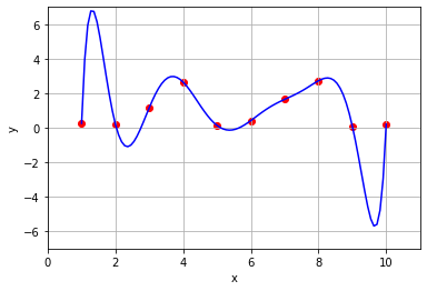
Judging by the graph of the polynomial, it looks like the curve takes on a value of about 2.5 when \(x = 3.5\) and a value of about 1 when \(x = 4.5\).
Although this method of finding a polynomial that passes through all our data points provides a nice smooth curve, it doesn’t match our intuition of what the curve should look like. The curve drops below zero between the ninth and tenth measurement, indicating a negative density. But this is impossible, since we can’t have a negative number of hares! It also rises much higher between the first and second measurement than the data points alone seem to suggest.
Exercise 2: The further you travel out into the solar system and away from the Sun, the slower an object must be travelling to remain in its orbit. Here are the average radii of the orbits of the planets in our solar system, and their average orbital velocity around the Sun.
Planet |
Distance from Sun (million km) |
Orbital Velocity (km/s) |
|---|---|---|
Mercury |
57.9 |
47.4 |
Venus |
108.2 |
35.0 |
Earth |
149.6 |
29.8 |
Mars |
228.0 |
24.1 |
Jupiter |
778.5 |
13.1 |
Saturn |
1432.0 |
9.7 |
Uranus |
2867.0 |
6.8 |
Neptune |
4515.0 |
5.4 |
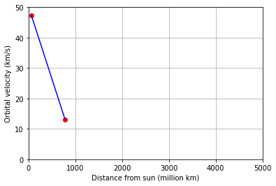
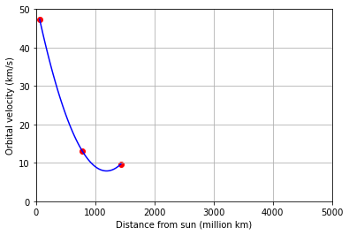
\((a)\) Find the unique first degree polynomial whose graph passes through points defined by Mercury and Jupiter. Plot the data points together with the graph of the polynomial to observe the fit. Amend your polynomial and graph by adding Saturn, and then Earth. What do you notice as you add more points? What if you had started with different planets?
\((b)\) Expand your work in part \((a)\) to a seventh degree poynomial that passes through all eight planets. The first object in the Kuiper Belt, Ceres, was discovered by Giuseppe Piazzi in 1801. Ceres has an average distance from the sun of 413.5 million km. Based on the points on the graph, estimate the orbital velocity of Ceres. What does the polynomial suggest the value would be?
We start by finding the polynomial and graph that passes through the points defined by Mercury and Jupiter.
x = np.array([57.9,778.5])
y = np.array([47.4,13.1])

A = np.zeros((2,2))
B = np.zeros((2,1))

for i in range(2):
    B[i,0] = y[i]
    for j in range(2):
        A[i,j] = x[i]**(j)

coeffs = lag.SolveSystem(A,B)

x_fit = np.linspace(x[0],x[1])
y_fit = coeffs[0] + coeffs[1]*x_fit
fig,ax = plt.subplots()

ax.scatter(x,y,color='red');
ax.plot(x_fit,y_fit,'b');
ax.set_xlim(0,5000);
ax.set_ylim(0,50);
ax.set_xlabel('Distance from sun (million km)');
ax.set_ylabel('Orbital velocity (km/s)');
ax.grid(True);
Next we add the point defined by Saturn.
x = np.array([57.9,778.5,1432.0])
y = np.array([47.4,13.1,9.7])

A = np.zeros((3,3))
B = np.zeros((3,1))

for i in range(3):
    B[i,0] = y[i]
    for j in range(3):
        A[i,j] = x[i]**(j)

coeffs = lag.SolveSystem(A,B)

x_fit = np.linspace(x[0],x[2])
y_fit = coeffs[0] + coeffs[1]*x_fit + coeffs[2]*x_fit**2
fig,ax = plt.subplots()

ax.scatter(x,y,color='red');
ax.plot(x_fit,y_fit,'b');
ax.set_xlim(0,5000);
ax.set_ylim(0,50);
ax.set_xlabel('Distance from sun (million km)');
ax.set_ylabel('Orbital velocity (km/s)');
ax.grid(True);
Next we add the point defined by Earth.
x = np.array([57.9,149.6,778.5,1432.0])
y = np.array([47.4,29.8,13.1,9.7])

A = np.zeros((4,4))
B = np.zeros((4,1))

for i in range(4):
    B[i,0] = y[i]
    for j in range(4):
        A[i,j] = x[i]**(j)

coeffs = lag.SolveSystem(A,B)

x_fit = np.linspace(x[0],x[3])
y_fit = coeffs[0] + coeffs[1]*x_fit + coeffs[2]*x_fit**2 + coeffs[3]*x_fit**3
fig,ax = plt.subplots()

ax.scatter(x,y,color='red');
ax.plot(x_fit,y_fit,'b');
ax.set_xlim(0,5000);
ax.set_ylim(0,50);
ax.set_xlabel('Distance from sun (million km)');
ax.set_ylabel('Orbital velocity (km/s)');
ax.grid(True);
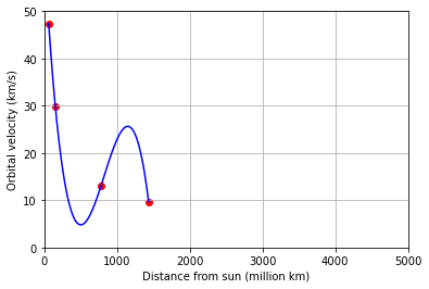
The polynomial seems to have a smoother, more “natural” curve when there are fewer points, but quickly overshoots as more points are added. Finally we extend the polynomial to fill all the points in the table.
x = np.array([57.9,108.2,149.6,228.0,778.5,1432.0,2867.0,4515.0])
y = np.array([47.4,35.0,29.8,24.1,13.1,9.7,6.8,5.4])


A = np.zeros((8,8))
B = np.zeros((8,1))

for i in range(8):
    B[i,0] = y[i]
    for j in range(8):
        A[i,j] = x[i]**(j)

coeffs = lag.SolveSystem(A,B)

x_fit = np.linspace(x[0],x[7])
y_fit = coeffs[0] + coeffs[1]*x_fit + coeffs[2]*x_fit**2 + coeffs[3]*x_fit**3 + coeffs[4]*x_fit**4 + coeffs[5]*x_fit**5 + coeffs[6]*x_fit**6 + coeffs[7]*x_fit**7

fig,ax = plt.subplots()

ax.scatter(x,y,color='red');
ax.plot(x_fit,y_fit,'b');
ax.set_xlim(0,5000);
ax.set_ylim(0,50);
ax.set_xlabel('Distance from sun (million km)');
ax.set_ylabel('Orbital velocity (km/s)');
ax.grid(True);
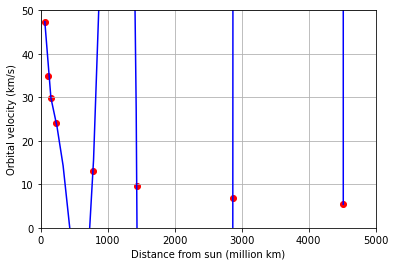
The polynomial looks like it takes on a value near 0 when \(x = 413.5\), but the points suggest something closer to 18.