Linear Systems
In this first chapter, we examine linear systems of equations and seek a method for their solution. We also introduce the machinery of matrix algebra which will be necessary in later chapters, and close with some applications.
A linear system of \(m\) equations with \(n\) unknowns \(x_1\), \(x_2\), \(x_3\), … \(x_n\), is a collection of equations that can be written in the following form.
Solutions to the linear system are collections of values for the unknowns that satisfy all of the equations simultaneously. The set of all possible solutions for the system is known as its solution set. A linear system that has at least one solution is said to be consistent, while a linear system that has no solutions is said to be inconsistent.
Linear systems with two equations and two unknowns are a great starting point since we easily graph the sets of points that satisfy each equation in the \(x_1x_2\) coordinate plane. The set of points that satisfy a single linear equation in two variables forms a line in the plane. Three examples will be sufficient to show the possible solution sets for linear systems in this setting.
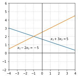
Example 1: System with a unique solution
The solution set for each equation can be represented by a line, and the solution set for the linear system is represented by all points that lie on both lines. In this case the lines intersect at a single point and there is only one pair of values that satisfy both equations, \(x_1 = -1\), \(x_2 = 2\). This linear system is consistent.
%matplotlib inline
import numpy as np
import matplotlib.pyplot as plt

x=np.linspace(-5,5,100)

fig, ax = plt.subplots()
ax.plot(x,(5-x)/3)
ax.plot(x,(5+x)/2)

ax.text(1,1.6,'$x_1+3x_2 = 5$')
ax.text(-3,0.5,'$x_1-2x_2 = -5$')

ax.set_xlim(-4,4)
ax.set_ylim(-2,6)
ax.axvline(color='k',linewidth = 1)
ax.axhline(color='k',linewidth = 1)

## This options specifies the ticks based the list of numbers provided.
ax.set_xticks(list(range(-4,5)))
ax.set_aspect('equal')
ax.grid(True,ls=':')
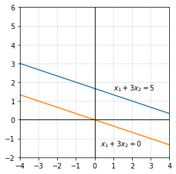
Example 2: System with no solutions
In this example the solution sets of the individual equations represent lines that are parallel. There is no pair of values that satisfy both equations simultaneously. This linear system is inconsistent.
fig, ax = plt.subplots()
ax.plot(x,(5-x)/3)
ax.plot(x,-x/3)

ax.text(1,1.6,'$x_1+3x_2 = 5$')
ax.text(0.3,-1.4,'$x_1+3x_2 = 0$')

ax.set_xlim(-4,4)
ax.set_ylim(-2,6)
ax.axvline(color='k',linewidth = 1)
ax.axhline(color='k',linewidth = 1)

## This options specifies the ticks based the list of numbers provided.
ax.set_xticks(list(range(-4,5)))
ax.set_aspect('equal')
ax.grid(True,ls=':')
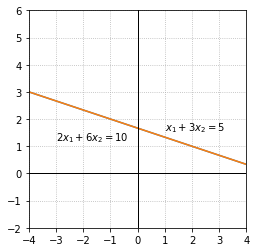
Example 3: System with an infinite number of solutions
In the final example, the second equation is a multiple of the first equation. The solution set for both equations is represented by the same line and thus every point on the line is a solution to the linear system. This linear system is consistent.
fig, ax = plt.subplots()
ax.plot(x,(5-x)/3)
ax.plot(x,(5-x)/3)

ax.text(1,1.6,'$x_1+3x_2 = 5$')
ax.text(-3,1.2,'$2x_1+6x_2 = 10$')

ax.set_xlim(-4,4)
ax.set_ylim(-2,6)
ax.axvline(color='k',linewidth = 1)
ax.axhline(color='k',linewidth = 1)

ax.set_xticks(list(range(-4,5)))
ax.set_aspect('equal')
ax.grid(True,ls=':')
These examples illustrate all of the possibile types of solution sets that might arise in a system of two equations with two unknowns. Either there will be exactly one solution, no solutions, or an infinite collection of solutions. A fundamental fact about linear systems is that their solution sets are always one of these three cases.
Exercises
Exercise 1: Consider the system of equations given below. Find a value for the coefficient \(a\) so that the system has exactly one solution. For that value of \(a\), find the solution to the system of equations and plot the lines formed by your equations to check your answer.
## Code solution here.
Exercise 2: Find a value for the coefficient \(a\) so that the system has no solution. Plot the lines formed by your equations to verify there is no solution.
## Code solution here.
Exercise 3: Consider the system of equations given below. Under what conditions on the coefficients \(a,b,c,d,e,f\) does this system have only one solution? No solutions? An infinite number of solutions? (Think about what must be true of the slopes and intercepts of the lines in each case.)
## Code solution here.