Vector Spaces
This chapter contain several concepts related to the the idea of a vector space. The main objective of the chapter is to tie these concepts to linear systems.
A vector space is a collection of objects, called vectors, together with definitions that allow for the addition of two vectors and the multiplication of a vector by a scalar. These operations produce other vectors in the collection and they satisfy a list of algebraic requirements such as associativity and commutativity. Although we will not consider the implications of each requirement here, we provide the list for reference.
For any vectors \(U\), \(V\), and \(W\), and scalars \(p\) and \(q\), the definitions of vector addition and scalar multiplication for a vector space have the following properties:
\(U+V = V+U\)
\((U+V)+W = U+(V+W)\)
\(U + 0 = U\)
\(U + (-U) = 0\)
\(p(qU) = (pq)U\)
\((p+q)U = pU + qU\)
\(p(U+V) = pU + pV\)
\(1U = U\)
The most familar example of vector spaces are the collections of single column arrays that we have been referring to as “vectors” throughout the previous chapter. The name given to the collection of all \(n\times 1\) arrays is known as Euclidean \(n\)-space, and is given the symbol \(\mathbb{R}^n\). The required definitions of addition and scalar multiplication in \(\mathbb{R}^n\) are those described for matrices in Matrix Algebra. We will leave it to the reader to verify that these operations satisfy the list of requirements listed above.
The algebra of vectors can be visualized by interpreting the vectors as arrows. This is easiest to see with an example in \(\mathbb{R}^2\).
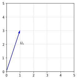
The vector \(U_1\) can be visualized as an arrow that points in the direction defined by 1 unit to the right, and 3 units up.
%matplotlib inline
import numpy as np
import matplotlib.pyplot as plt

fig, ax = plt.subplots()
options = {"head_width":0.1, "head_length":0.2, "length_includes_head":True}

ax.arrow(0,0,1,3,fc='b',ec='b',**options)

ax.text(1,2,'$U_1$')

ax.set_xlim(0,5)
ax.set_ylim(0,5)
ax.set_aspect('equal')
ax.grid(True,ls=':')
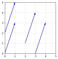
It is important to understand that it is the length and direction of this arrow that defines \(U_1\), not the actual position. We could draw the arrow in any number of locations, and it would still represent \(U_1\).
fig, ax = plt.subplots()

ax.arrow(0,0,1,3,fc='b',ec='b',**options)
ax.arrow(3,0,1,3,fc='b',ec='b',**options)
ax.arrow(0,2,1,3,fc='b',ec='b',**options)
ax.arrow(2,1,1,3,fc='b',ec='b',**options)

ax.set_xlim(0,5)
ax.set_ylim(0,5)
ax.set_aspect('equal')
ax.grid(True,ls=':')
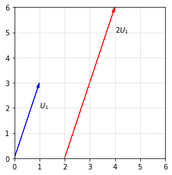
When we perform a scalar multiplication, such as \(2U_1\), we interpret it as multiplying the length of the arrow by the scalar.
fig, ax = plt.subplots()

ax.arrow(0,0,1,3,fc='b',ec='b',**options)
ax.arrow(2,0,2,6,fc='r',ec='r',**options)

ax.text(1,2,'$U_1$')
ax.text(4,5,'$2U_1$')

ax.set_xlim(0,6)
ax.set_ylim(0,6)
ax.set_aspect('equal')
ax.grid(True,ls=':')

ax.set_xticks(np.arange(0,7,step = 1));
ax.set_yticks(np.arange(0,7,step = 1));
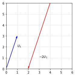
If the scalar is negative, we interpret the scalar multiplication as reversing the direction of the arrow, as well as changing the length.
fig, ax = plt.subplots()

ax.arrow(0,0,1,3,fc='b',ec='b',**options)
ax.arrow(4,6,-2,-6,fc='r',ec='r',**options)

ax.text(1,2,'$U_1$')
ax.text(3,1,'$-2U_1$')

ax.set_xlim(0,6)
ax.set_ylim(0,6)
ax.set_aspect('equal')
ax.grid(True,ls=':')

ax.set_xticks(np.arange(0,7,step = 1));
ax.set_yticks(np.arange(0,7,step = 1));
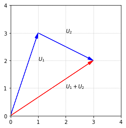
We can interpret the sum of two vectors as the result of aligning the two arrows tip to tail.
fig, ax = plt.subplots()

ax.arrow(0,0,1,3,fc='b',ec='b',**options)
ax.arrow(1,3,2,-1,fc='b',ec='b',**options)
ax.arrow(0,0,3,2,fc='r',ec='r',**options)

ax.text(1,2,'$U_1$')
ax.text(2,3,'$U_2$')
ax.text(2,1,'$U_1+U_2$')

ax.set_xlim(0,4)
ax.set_ylim(0,4)
ax.set_aspect('equal')
ax.grid(True,ls=':')

ax.set_xticks(np.arange(0,5,step = 1));
ax.set_yticks(np.arange(0,5,step = 1));
There are many other examples of vector spaces, but we will wait to provide these until after we have discussed more of the fundamental vector space concepts using \(\mathbb{R}^n\) as the setting.