Transformations in a Plane
As discussed in the previous section, any linear transformation \(T:\mathbb{R}^2\to\mathbb{R}^2\) can be represented as the multiplication of a \(2\times 2\) matrix and a coordinate vector. For now, the coordinates are with respect to the standard basis \(\{E_1,E_2\}\) as they were before. The columns of the matrix are then the images of the the basis vectors.
Example 1: Horizontal Stretch
As a first example let us consider the transformation defined by the following images.
The matrix corresponding to the transformation is then
The image of a general vector with components \(c_1\) and \(c_2\) is given by a linear combination of the images of the basis vectors.
To get a visual understanding of the transformation, we produce a plot that displays multiple input vectors, and their corresponding images. Since we will multiply each vector by the same matrix, we can organize our calculations by constructing a matrix with columns that match the input vectors. This matrix is the array labeled \(\texttt{coords}\) in the code below. We use array slicing to label the first row \(\texttt{x}\), and the second row \(\texttt{y}\) for the purposes of plotting.
%matplotlib inline
from math import pi, sin, cos
import matplotlib.pyplot as plt
import numpy as np

coords = np.array([[0,0],[0.5,0.5],[0.5,1.5],[0,1],[0,0]])
coords = coords.transpose()
coords
x = coords[0,:]
y = coords[1,:]

A = np.array([[2,0],[0,1]])
A_coords = A@coords
The columns of the array \(\texttt{A_coords}\) are the images of the vectors that make up the columns of \(\texttt{coords}\). Let’s plot the coordinates and see the effect of the transformation. Again, we need to access the first and second rows by slicing. The red points show the original coordinates, and the new coordinates are shown in blue.
x_LT1 = A_coords[0,:]
y_LT1 = A_coords[1,:]

# Create the figure and axes objects
fig, ax = plt.subplots()

# Plot the points.  x and y are original vectors, x_LT1 and y_LT1 are images
ax.plot(x,y,'ro')
ax.plot(x_LT1,y_LT1,'bo')

# Connect the points by lines
ax.plot(x,y,'r',ls="--")
ax.plot(x_LT1,y_LT1,'b')

# Edit some settings
ax.axvline(x=0,color="k",ls=":")
ax.axhline(y=0,color="k",ls=":")
ax.grid(True)
ax.axis([-2,2,-1,2])
ax.set_aspect('equal')
ax.set_title("Horizontal Stretch");
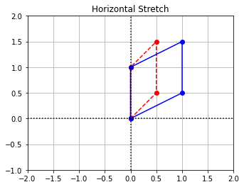
We observe that the result of the transformation is that the polygon has been stretched in the horizontal direction.
Example 2: Reflection
Now that we have a set of vectors stored in the \(\texttt{coords}\) matrix, let’s look at another transformation that is defined by the matrix \(B\).
We make a new array \(B\), but reuse the plotting code from the previous example.
B = np.array([[-1,0],[0,1]])
B_coords = B@coords

x_LT2 = B_coords[0,:]
y_LT2 = B_coords[1,:]

# Create the figure and axes objects
fig, ax = plt.subplots()

# Plot the points.  x and y are original vectors, x_LT1 and y_LT1 are images
ax.plot(x,y,'ro')
ax.plot(x_LT2,y_LT2,'bo')

# Connect the points by lines
ax.plot(x,y,'r',ls="--")
ax.plot(x_LT2,y_LT2,'b')

# Edit some settings
ax.axvline(x=0,color="k",ls=":")
ax.axhline(y=0,color="k",ls=":")
ax.grid(True)
ax.axis([-2,2,-1,2])
ax.set_aspect('equal')
ax.set_title("Reflection");
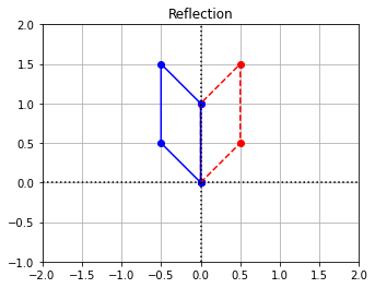
We see that this transformation reflects points around the vertical axis.
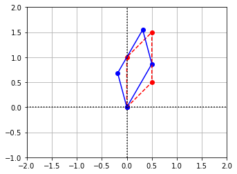
Example 3: Rotation
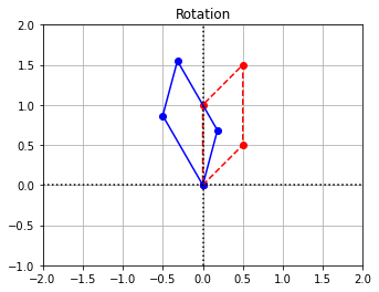
To rotate vectors in the plane, we choose an angle \(\theta\) and write down the matrix that represents the rotation counterclockwise by an angle \(\theta\). Basic trigonometry can be used to calculate the columns in this case.
theta = pi/6
R = np.array([[cos(theta),-sin(theta)],[sin(theta),cos(theta)]])
R_coords = R@coords

x_LT3 = R_coords[0,:]
y_LT3 = R_coords[1,:]

# Create the figure and axes objects
fig, ax = plt.subplots()

# Plot the points.  x and y are original vectors, x_LT1 and y_LT1 are images
ax.plot(x,y,'ro')
ax.plot(x_LT3,y_LT3,'bo')

# Connect the points by lines
ax.plot(x,y,'r',ls="--")
ax.plot(x_LT3,y_LT3,'b')

# Edit some settings
ax.axvline(x=0,color="k",ls=":")
ax.axhline(y=0,color="k",ls=":")
ax.grid(True)
ax.axis([-2,2,-1,2])
ax.set_aspect('equal')
ax.set_title("Rotation");
Example 4: Shear
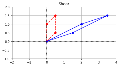
In the study of mechanics, shear forces occur when one force acts on some part of a body while a second force acts on another part of the body but in the opposite direction. To visualize this, imagine a deck of playing cards resting on the table, and then while resting your hand on top of the deck, sliding your hand parallel to the table.
A shear transformation is any transformation that shifts points in a given direction by an amount proportional to their original (signed) distance from the line that is parallel to the movement of direction and that passes through the origin. For example, a horizontal shear applied to a vector would add to the vector’s \(x\)-coordinate a value scaled by the value of its \(y\)-coordinate (or subtract, if the \(y\)-coordinate was negative). A vertical shear is expressed as a matrix in the form of the first matrix below, and a horizontal shear with the second where \(k \in \mathbb{R}\) is called the shearing factor.
S = np.array([[1,2],[0,1]])
S_coords = S@coords

x_LT4 = S_coords[0,:]
y_LT4 = S_coords[1,:]


# Create the figure and axes objects
fig, ax = plt.subplots()

# Plot the points.  x and y are original vectors, x_LT1 and y_LT1 are images
ax.plot(x,y,'ro')
ax.plot(x_LT4,y_LT4,'bo')

# Connect the points by lines
ax.plot(x,y,'r',ls="--")
ax.plot(x_LT4,y_LT4,'b')

# Edit some settings
ax.axvline(x=0,color="k",ls=":")
ax.axhline(y=0,color="k",ls=":")
ax.grid(True)
ax.axis([-2,4,-1,2])
ax.set_aspect('equal')
ax.set_title("Shear");
Example 5: Composition of transformations
One of the powerful aspects of representing linear transformations as matrices is that we can form compositions by matrix multiplication. For example, in order to find the matrix that represents the composition \(B\circ R\), the rotation from Example 3, followed by the reflection of Example 2, we can simply multiply the matrices that represent the individual transformations.
C = np.array([[-cos(theta),sin(theta)],[sin(theta),cos(theta)]])
C_coords = C@coords

x_LT5 = C_coords[0,:]
y_LT5 = C_coords[1,:]


# Create the figure and axes objects
fig, ax = plt.subplots()

# Plot the points.  x and y are original vectors, x_LT1 and y_LT1 are images
ax.plot(x,y,'ro')
ax.plot(x_LT5,y_LT5,'bo')

# Connect the points by lines
ax.plot(x,y,'r',ls="--")
ax.plot(x_LT5,y_LT5,'b')

# Edit some settings
ax.axvline(x=0,color="k",ls=":")
ax.axhline(y=0,color="k",ls=":")
ax.grid(True)
ax.axis([-2,2,-1,2])
ax.set_aspect('equal')
Exercises
Exercise 1:
(\(a\)) Find a matrix that represents the reflection about the \(x_1\)-axis.
## Code solution here.
(\(b\)) Multiply the matrix by \(\texttt{coords}\) and plot the results.
## Code solution here.
Exercise 2:
(\(a\)) Find a matrix that represents the reflection about the line \(x_1=x_2\).
## Code solution here.
(\(b\)) Multiply the matrix by \(\texttt{coords}\) and plot the results.
## Code solution here.
Exercise 3:
(\(a\)) Find a matrix that represents the rotation clockwise by an angle \(\theta\).
## Code solution here.
(\(b\)) Let \(\theta = 90^{\circ}\). Multiply the matrix by \(\texttt{coords}\) and plot the results.
## Code solution here.
Exercise 4:
(\(a\)) Find a matrix that represents a vertical shear followed by the rotation in Example 3.
## Code solution here.
(\(b\)) Multiply the matrix by \(\texttt{coords}\) and plot the results.
## Code solution here.
Exercise 5: Create a new matrix of coordinates and apply one of the transformations in the Examples. Plot the results.
## Code solution here.
Exercise 6:
(\(a\)) Construct a matrix that represents a horizontal and a vertical stretch by a factor of 2 .
## Code solution here
(\(b\)) Create a new matrix of coordinates. Apply this transformation and plot the results.
## Code solution here