Eigenvalues
import laguide as lag
import numpy as np
import scipy.linalg as sla
%matplotlib inline
import matplotlib.pyplot as plt
import math
Exercise 1: Determine the eigenvalues and corresponding eigenvectors of the following matrices by considering the transformations that they represent. Check your answers with a few computations.
\((a)\)
Solution:
Recall from Chapter 4 that applying the transformation represented by \(A\) is equivalent to stretching in the direction of the \(y\)-axis by a factor of 3 and then reflecting over the \(y\)-axis. If we imagine what this does to vectors in the plane then we might see that any vector that lies on the \(x\)-axis will be left unaffected. Therefore our first eigenvalue is \(\lambda_1 = 1\) which corresponds to any scalar multiple of our first eigenvector \(V_1 = \begin{equation} \left[ \begin{array}{cc} 1 \\ 0 \end{array}\right] \end{equation}\). Additionally, any vector that lies on the \(y\)-axis will simply be scaled by a factor of \(-3\). Therefore our second eigenvalue is \(\lambda_2 = -3\) which corresponds to any scalar multiple of our second eigenvector \(V_2 = \begin{equation} \left[ \begin{array}{cc} 0 \\ 1 \end{array}\right] \end{equation}\).
A = np.array([[1,0],[0,-3]])
V1 = np.array([[1],[0]])
V2 = np.array([[0],[1]])
R = np.array([[5],[0]])
S = np.array([[1],[1]])
T = np.array([[0],[0]])

print(A@V1,'\n')
print(A@V2,'\n')
print(A@R,'\n')
print(A@S,'\n')
print(A@T)
[[1]
 [0]]

[[ 0]
 [-3]]

[[5]
 [0]]

[[ 1]
 [-3]]

[[0]
 [0]]
\((b)\)
Solutions:
Recall from Chapter 4 that applying the transformation represented by \(B\) is equivalent to shearing along the \(x\)-axis with a shearing factor of 1. Any vector that lies along the \(x\)-axis will be left unchanged because its \(y\)-coordinate is 0 and thus adds nothing to \(x\)-coordinate. Therefore our first eigenvalue is \(\lambda_1 = 1\) which corresponds to any scalar multiple of our first eigenvector \(V_1 = \begin{equation} \left[ \begin{array}{cc} 1 \\ 0 \end{array}\right] \end{equation}\). Any other vector with a nonzero \(y\)-coordinate will shear off of its original span, and thus cannot be a scalar multiple of itself. Therefore \(V_1\) is the only eigenvalue of \(B\).
B = np.array([[1,1],[0,1]])
V1 = np.array([[1],[0]])
V2 = np.array([[0],[1]])
R = np.array([[5],[0]])
S = np.array([[1],[1]])
T = np.array([[0],[0]])

print(B@V1,'\n')
print(B@V2,'\n')
print(B@R,'\n')
print(B@S,'\n')
print(B@T)
[[1]
 [0]]

[[1]
 [1]]

[[5]
 [0]]

[[2]
 [1]]

[[0]
 [0]]
\((c)\)
Solution:
Recall from Chapter 4 that applying the transformation represented by \(C\) is equivalent to a rotation about the origin by the angle \(\frac{\pi}{2}\). Any nonzero vector that is transformed by this matrix will be pointing directly perpendicular to its original direction, so cannot lie on its original span. Therefore \(C\) has no eigenvalues nor any eigenvectors.
C = np.array([[math.cos(math.pi/2),-math.sin(math.pi/2)],[math.sin(math.pi/2),math.cos(math.pi/2)]])
V1 = np.array([[1],[0]])
V2 = np.array([[0],[1]])
R = np.array([[5],[0]])
S = np.array([[1],[1]])
T = np.array([[0],[0]])

print(np.round(C@V1),'\n')
print(np.round(C@V2),'\n')
print(np.round(C@R),'\n')
print(np.round(C@S),'\n')
print(np.round(C@T))
[[0.]
 [1.]]

[[-1.]
 [ 0.]]

[[0.]
 [5.]]

[[-1.]
 [ 1.]]

[[0.]
 [0.]]
\((d)\)
Solution: If we plot a shape before and after applying this transformation, it appears that this matrix reflects over the line \(y=-2x\).
coords = np.array([[0,0],[1,0],[1,1],[0,1],[0,0]])
coords = coords.transpose()
D = np.array([[-0.6,-0.8],[-0.8,0.6]])
D_coords = D@coords

x = coords[0,:]
y = coords[1,:]
x_LT = D_coords[0,:]
y_LT = D_coords[1,:]

# Create the figure and axes objects
fig, ax = plt.subplots()

# Plot the points and the line y = -2x. x and y are original vectors, x_LT and y_LT are images
ax.plot(x,y,'ro')
ax.plot(x_LT,y_LT,'bo')
a=np.linspace(-2,2,100)
ax.plot(a,-2*a,ls=':')

# Connect the points by lines
ax.plot(x,y,'r',ls="--")
ax.plot(x_LT,y_LT,'b')

# Edit some settings
ax.axvline(x=0,color="k",ls=":")
ax.axhline(y=0,color="k",ls=":")
ax.grid(True)
ax.axis([-2,2,-1,2])
ax.set_aspect('equal')
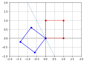
Any vector that lies on the line \(y = -2x\) will be left unchanged, so our first eigenvalue is \(\lambda_1 = 1\) which corresponds to any scalar multiple of our first eigenvector \(V_1 = \begin{equation} \left[ \begin{array}{cc} 1 \\ -2 \end{array}\right] \end{equation}\). Any vector that lies on the line orthogonal to the first, namely \(y = \frac{1}{2}x\) will be simply flipped in direction, or in other words scaled by a factor of \(-1\). Thus our second eigenvalue is \(\lambda_2 = -1\) which corresponds to any scalar multiple of our second eigenvector \(V_2 = \begin{equation} \left[ \begin{array}{cc} 2 \\ 1 \end{array}\right] \end{equation}\).
D = np.array([[-0.6,-0.8],[-0.8,0.6]])
V1 = np.array([[1],[-2]])
V2 = np.array([[2],[1]])
R = np.array([[5],[0]])
S = np.array([[1],[1]])
T = np.array([[0],[0]])

print(D@V1,'\n')
print(D@V2,'\n')
print(D@R,'\n')
print(D@S,'\n')
print(D@T)
[[ 1.]
 [-2.]]

[[-2.]
 [-1.]]

[[-3.]
 [-4.]]

[[-1.4]
 [-0.2]]

[[0.]
 [0.]]
Exercise 2: Find the eigenvalues and the corresponding eigenvectors of the following matrix \(R\) that represents the reflection transformation about the line \( x_1 = x_2 \).
Solution:
Let us consider the vector \( V_1\) as follows:
We can see that \( RV_1 = V_1\). So, \(\lambda_1 = 1\) is one of the eigenvalues of \(R\).
Similarly, let us consider the vector \(V_2\) as follows:
We observe that \(RV_2 = -V_2\).
So, \(\lambda_2 = -1\) is another eigenvalue of \(R\).
Therefore, we can say that there are two eigenvalues of the matrix \(R\) i.e \(\lambda_1 = 1\), \(\lambda_2 = -1\). The vector \(V_1\) and all its scalar multiples are eigenvectors associated with \(\lambda_1\), \(V_2\) and all its scalar multiples are eigenvectors associated with \(\lambda_2\).
## Building matrix R and vectors V_1,V_2:

V_1 = np.array([[1],[1]])
V_2 = np.array([[1],[-1]])
R = np.array([[0,1],[1,0]])

print("RV_1: \n", R@V_1, '\n')
print("RV_2: \n", R@V_2, '\n')
RV_1:
 [[1]
 [1]]

RV_2:
 [[-1]
 [ 1]]
Exercise 3: Find a matrix that represents a vertical and horizontal stretch by a factor of \(2\). Then, find the eigenvalues and the eigenvectors associated with those eigenvalues. (You may have to take a look at the Planar Transformations section Planar Transformations).
Solution:
Based on our discussion on Planar Transformations, the matrix that represents a vertical stretch and horizontal stretch is as follows:
Since the effect of the transformation is to scale all vectors by a factor of \(2\), all vectors are eigenvectors of the matrix \(A\).
Let us consider the vector \(V_1\) as an example.
We can see that \(AV_1 = 2V_1\). The only eigenvalue of \(A\) is \(2\).
## building matrix A and vectors V_1, V_2:

A = np.array([[2,0],[0,2]])
V_1 = np.array([[1],[1]])
V_2 = np.array([[1],[0]])

print("AV_1: \n", A@V_1, '\n')
print("AV_2: \n", A@V_2, '\n')
AV_1:
 [[2]
 [2]]

AV_2:
 [[2]
 [0]]
Exercise 4: Find a matrix that represents reflection about the \(x_1-\)axis and find its eigenvalues and eigenvectors.
Solution:
Based on our discussion on Planar Transformations, the matrix that represents reflection about the \(x_1\) -axis is as follows:
Let us consider the vector \(V_1\) as follows:
Since \(BV_1 = V_1\), one of the eigenvalues of the matrix \(B\) is \(\lambda_1 = 1\) and \(V_1\) is the eigenvector associated with \(\lambda_1\). Infact, all the scalar multiples of \(V_1\) are also eigenvectors associated with \(\lambda_1\).
Now, let us consider another vector \(V_2\) as follows:
Since \(BV_2 = -V_2\), other eigenvalue for the matrix \(B\) will be \(\lambda_2 =-1\) and \(V_2\) is the eigenvector associated with \(\lambda_2\). All the scalar multiples of \(V_2\) are also eigenvectors associated with \(\lambda_2\).
## Building the matrix B and the vectors V_1, V_2:

B = np.array([[1,0],[0,-1]])
V_1 = np.array([[1],[0]])
V_2 = np.array([[0],[1]])

print("BV_1: \n", B@V_1, '\n')
print("BV_2: \n", B@V_2, '\n')
BV_1:
 [[1]
 [0]]

BV_2:
 [[ 0]
 [-1]]
Diagonalization
Exercise 1: Find the diagonalization of the matrix from Example 1.
Solution: Recall that \(A\) has eigenvalues \(\lambda_1 = 3\) and \(\lambda_2 = 1\), and corresponding eigenvectors \(V_1\) and \(V_2\) defined below.
To find the diagonalization of \(A\), we need to find the diagonal matrix \(D\) with the eigenvalues of \(A\) along its diagonal, and the matrix \(S\) which has columns equal to the eigenvectors of \(A\). We write them out below, and then verify that \(A = SDS^{-1}\).
A = np.array([[2,-1],[-1,2]])
D = np.array([[3,0],[0,1]])
S = np.array([[1,1],[-1,1]])
print(A - S@D@lag.Inverse(S))
[[0. 0.]
 [0. 0.]]
Exercise 2: Find the diagonalization of the following matrix.
Solution: First we must find the eigenvectors of \(B\) and their corresponding eigenvalues. We make use of the \(\texttt{eig}\) function to do this.
B = np.array([[2,0,0],[3,-2,1],[1,0,1]])
evalues,evectors = sla.eig(B)
print(evalues,'\n')
print(evectors)
[-2.+0.j  1.+0.j  2.+0.j]

[[0.         0.         0.57735027]
 [1.         0.31622777 0.57735027]
 [0.         0.9486833  0.57735027]]
\(S\) is equivalent to the matrix of eigenvectors above, so all we have to do is write out \(D\) and then verify that \(B = SDS^{-1}\).
D = np.array([[-2,0,0],[0,1,0],[0,0,2]])
S = evectors
print(B - S@D@lag.Inverse(S))
[[0.00000000e+00 0.00000000e+00 0.00000000e+00]
 [0.00000000e+00 0.00000000e+00 0.00000000e+00]
 [1.11022302e-16 0.00000000e+00 0.00000000e+00]]
Exercise 3: Write a function that accepts an \(n\times n\) matrix \(A\) as an argument, and returns the three matrices \(S\), \(D\), and \(S^{-1}\) such that \(A=SDS^{-1}\). Make use of the \(\texttt{eig}\) function in SciPy.
Solution: We write a function that finds the diagonalization of an \(n \times n\) matrix \(A\) and then test it on the matrix \(B\) defined in exercise 2 to check that it works.
def Diagonalization(A):
    '''
    Diagonalization(A)

    Diagonalization takes an nxn matrix A and computes the diagonalization
    of A. There is no error checking to ensure that the eigenvectors of A
    form a linearly independent set.

    Parameters
    ----------
    A : NumPy array object of dimension nxn

    Returns
    -------
    S :        NumPy array object of dimension nxn
    D :        NumPy array object of dimension nxn
    S_inverse: Numpy array object of dimension nxn
    '''

    n = A.shape[0]  # n is number of rows and columns in A
    D = np.zeros((3,3),dtype='complex128')
    evalues,evectors = sla.eig(A)

    S = evectors
    S_inverse = lag.Inverse(S)

    for i in range(0,n,1):
        D[i][i] = evalues[i]

    return S,D,S_inverse

B = np.array([[2,0,0],[3,-2,1],[1,0,1]])
S, D, S_inverse = Diagonalization(B)
print(S,'\n')
print(D,'\n')
print(S_inverse)
[[0.         0.         0.57735027]
 [1.         0.31622777 0.57735027]
 [0.         0.9486833  0.57735027]]

[[-2.+0.j  0.+0.j  0.+0.j]
 [ 0.+0.j  1.+0.j  0.+0.j]
 [ 0.+0.j  0.+0.j  2.+0.j]]

[[-0.66666667  1.         -0.33333333]
 [-1.05409255  0.          1.05409255]
 [ 1.73205081  0.          0.        ]]
Exercise 4: Construct a \(3\times 3\) matrix that is not diagonal and has eigenvalues 2, 4, and 10.
Solution: If we want to construct a matrix \(C\) with eigenvalues 2, 4, and 10, then \(D\) must be a diagonal matrix with those eigenvalues as its diagonal entries. If we let \(S\) be any \(3 \times 3\) non diagonal matrix with linearly independent columns, then \(C = SDS^{-1}\) will give us our desired matrix. We define \(D\) and \(S\) below, calculate \(C\), and then check our answer using the \(\texttt{eig}\) function.
D = np.array([[2,0,0],[0,4,0],[0,0,10]])
S = np.array([[1,1,0],[0,1,1],[1,0,1]])
C = S@D@lag.Inverse(S)

print(C,'\n')

evalues,evectors = sla.eig(C)
print(evalues)
[[ 3.  1. -1.]
 [-3.  7.  3.]
 [-4.  4.  6.]]

[10.+0.j  2.+0.j  4.+0.j]
The eigenvalues determined by \(\texttt{eig}\) appear in a different order than we had originally, but are correct.
Exercise 5: Suppose that \(C = QDQ^{-1}\) where
\((a)\) Give a basis for \(\mathcal{N}(C)\)
Solution: Consider the set \(\{U,V,W\}\). This set of three vectors is linearly independent, so it forms a basis for \(\mathbb{R}^3\) and thus any vector \(X \in \mathbb{R}^3\) can be expressed as a linear combination \(X = aU + bV +cW\) for some scalars \(a,b,\) and \(c\). Then we have
Since \(V\) and \(W\) are linearly independent, so are \(3V\) and \(5W\), and therefore the only way that \(b3V + c5W = 0\) is if \(b = c = 0\). This means that \(CX = 0\) when \(b = c = 0\) and there is no restriction on \(a\). But then any element in the null space of \(C\) can be expressed as a scalar multiple of \(U\) and thus \(\{U\}\) is a basis for \(\mathcal{N}(C)\).
\((b)\) Find all the solutions to \(CX = V + W\)
Solution: Let \(X\) be an arbitrary vector in \(\mathbb{R}^3\). Since the set of three vectors \(\{U,V,W\}\) are linearly independent, they form a basis for \(\mathbb{R}^3\), and thus we can write \(X = aU + bV + cW\) for some scalars \(a,b,\) and \(c\). Then we have
This whole thing is equal to \(V+W\) when \(b = \frac{1}{3}\), \(c = \frac{1}{5}\), and is independent of \(a\). Therefore the solutions to \(CX = V + W\) are the vectors of the form \(X = aU + \frac{1}{3}V + \frac{1}{5}W\) where \(a\) is any real number.
Approximating Eigenvalues
Exercise 1: Let \(A\) be the matrix from the Inverse Power Method example.
\((a)\) Use the Power Method to approximate the largest eigenvalue \(\lambda_1\). Verify that the exact value of \(\lambda_1\) is 12.
Solution:
A = np.array([[9,-1,-3],[0,6,0],[-6,3,6]])
X = np.array([[0],[1],[0]])

m = 0
tolerance = 0.0001
MAX_ITERATIONS = 100

## Compute difference in stopping condition
## Assign Y = AX to avoid computing AX multiple times
Y = A@X
difference = Y - lag.Magnitude(Y)*X

while (m < MAX_ITERATIONS and lag.Magnitude(difference) > tolerance):
    X = Y
    X = X/lag.Magnitude(X)

    ## Compute difference in stopping condition
    Y = A@X
    difference = Y - lag.Magnitude(Y)*X

    m = m + 1

print("Eigenvector is approximately:")
print(X,'\n')
print("Magnitude of the eigenvalue is approximately:")
print(lag.Magnitude(Y),'\n')
Eigenvector is approximately:
[[-7.07103544e-01]
 [ 9.71065612e-06]
 [ 7.07110018e-01]]

Magnitude of the eigenvalue is approximately:
12.000013732475342
It appears that the first entry of \(X\) is equal to the third multiplied by \(-1\). If we set the first entry to be 1 and the third entry to be -1, we can calculate the following product and see that \(\lambda_1\) is indeed 12.
\((b)\) Apply the Inverse Power Method with a shift of \(\mu = 10\). Explain why the results differ from those in the example.
Solution:
A = np.array([[9,-1,-3],[0,6,0],[-6,3,6]])
X = np.array([[0],[1],[0]])

m = 0
tolerance = 0.0001
MAX_ITERATIONS = 100
difference = X

A = np.array([[9,-1,-3],[0,6,0],[-6,3,6]])
I = np.eye(3)
mu = 10
Shifted_A = A-mu*I
LU_factorization = sla.lu_factor(Shifted_A)

while (m < MAX_ITERATIONS and lag.Magnitude(difference) > tolerance):
    X_previous = X
    X = sla.lu_solve(LU_factorization,X)
    X = X/lag.Magnitude(X)

    ## Compute difference in stopping condition
    difference = X - X_previous

    m = m + 1

print("Eigenvector is approximately:")
print(X,'\n')
print("Eigenvalue of A is approximately:")
print(lag.Magnitude(A@X))
Eigenvector is approximately:
[[-7.07113254e-01]
 [-1.94211789e-05]
 [ 7.07100308e-01]]

Eigenvalue of A is approximately:
11.99997253020264
The Inverse Power Method with a shift of \(\mu\) finds the eigenvalue closest to \(\mu\). \(A\) has three eigenvalues, namely 3, 6, and 12, of which 10 is closest to 12 and 7.5 is closest to 6. This is why when we used \(\lambda = 7.5\) in the example we got the eigenvalue 6, but when we used \(\lambda = 10\) we got the eigenvalue 12.
\((c)\) Apply the Inverse Power Method with a shift of \(\mu = 7.5\) and the initial vector given below. Explain why the sequence of vectors approach the eigenvector corresponding to \(\lambda_1\)
Solution:
## Code solution here.
Applications
Exercise 1: Experiment with a range of initial conditions in the infectious disease model to provide evidence that an equilibrium state is reached for all meaningful initial states.
We will create a method that uses the model given in the example but takes in a vector representing the initial conditions, then outputs the graphs of the values over time. We will input several different sets of intial conditions and graph them, verifying that they all seem to converge upon the same equilibrium state.
def Iterate_SIRS(X):

    A = np.array([[0.95, 0, 0.15],[0.05,0.8,0],[0,0.2,0.85]])

    ## T is final time
    T = 20

    ## The first column of results contains the initial values
    results = np.copy(X)

    for i in range(T):
        X = A@X
        results = np.hstack((results,X))

    ## t contains the time indices 0, 1, 2, ..., T
    t = np.linspace(0,T,T+1)
    ## s, i, r values are the rows of the results array
    s = results[0,:]
    i = results[1,:]
    r = results[2,:]

    fig,ax = plt.subplots()

    ## The optional label keyword argument provides text that is used to create a legend
    ax.plot(t,s,'b+',label="Susceptible");
    ax.plot(t,i,'rx',label="Infectious");
    ax.plot(t,r,'g+',label="Recovered");

    ax.set_ylim(0,1.1)
    ax.grid(True)
    ax.legend();

Iterate_SIRS(np.array([[0.95],[0.05],[0]]))
Iterate_SIRS(np.array([[0.7],[0.05],[0.25]]))
Iterate_SIRS(np.array([[0.3],[0.4],[0.3]]))
Iterate_SIRS(np.array([[0.1],[0.8],[0.1]]))
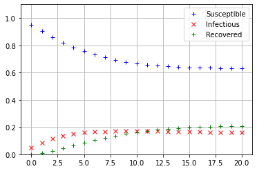
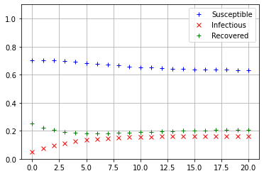
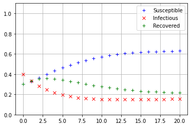
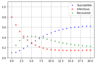
The values of \(s_{20}, i_{20},\) and \(r_{20}\) see to be nearly equal, so it appears that regardless of the initial conditions, the SIRS model always converges to the same equilibrium state.
Exercise 2: Perform an analysis similar to that in the example for the following infectious disease model. In this model the rate at which individuals move from the Recovered category to the Susceptible category is less than that in the example. Make a plot similar to that in the example and also calculate the theoretical equilibrium values for \(s\), \(i\), and \(r\).
We will plot the first 50 iterations of \(s_t,i_t,\) and \(r_t\) using the same initial conditions as the example.
A = np.array([[0.95, 0, 0.05],[0.05,0.8,0],[0,0.2,0.95]])

## T is final time
T = 50
## X at time 0
X = np.array([[0.95],[0.05],[0]])

## The first column of results contains the initial values
results = np.copy(X)

for i in range(T):
    X = A@X
    results = np.hstack((results,X))

## t contains the time indices 0, 1, 2, ..., T
t = np.linspace(0,T,T+1)
## s, i, r values are the rows of the results array
s = results[0,:]
i = results[1,:]
r = results[2,:]

fig,ax = plt.subplots()

## The optional label keyword argument provides text that is used to create a legend
ax.plot(t,s,'b+',label="Susceptible");
ax.plot(t,i,'rx',label="Infectious");
ax.plot(t,r,'g+',label="Recovered");

ax.set_ylim(0,1.1)
ax.grid(True)
ax.legend();
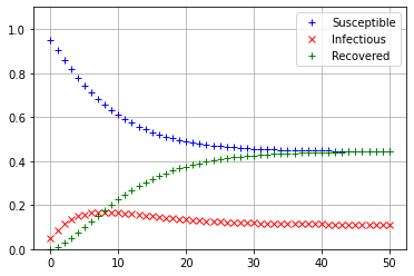
It appears that the population has reached an equilibrium after about 45 weeks, but one that was different than in the example. The proportion of the population that is susceptible seems to be equal to the porportion of the population that is recovered at roughly 45%, and the proportion that is infectious seems to be about 10%. To find the true equilibrium values, we calculate the \(\texttt{RREF}\) of the augmented matrix \([(A-I)|0]\).
I = np.eye(3)
ZERO = np.zeros((3,1))
augmented_matrix = np.hstack((A-I,ZERO))
reduced_matrix = lag.FullRowReduction(augmented_matrix)
print(reduced_matrix)
[[ 1.    0.   -1.    0.  ]
 [ 0.    1.   -0.25  0.  ]
 [ 0.    0.    0.    0.  ]]
In the reduced system for the equilibrium values \(s\), \(i\), and \(r\), we can take \(r\) as the free variable and write \(s=r\) and \(i=0.25r\). For any value of \(r\), a vector of the following form is an eigenvector for \(A-I\), corresponding to the eigenvalue one.
If we add the constraint that \(s + i + r = 1\), then we get the equation \(r + 0.25r + r = 1\) which gives the unique equilibrium values of \(r = 4/9\), \(s=4/9\), and \(i=1/9\). If we carry out a large number of iterations, we see that the computed values are very close to the theoretical equilibrium values.
## T is final time
T = 100
## X at time 0
X = np.array([[0.95],[0.05],[0]])

for i in range(T):
    X = A@X

print("Computed values of s, i, r at time ",T,":")
print(X)
Computed values of s, i, r at time  100 :
[[0.44444478]
 [0.1111114 ]
 [0.44444382]]