Linear Combinations
At the core of many ideas in linear algebra is the concept of a linear combination of vectors. To build a linear combination from a set of vectors \(\{V_1, V_2, V_3, ... V_n\}\) we use the two algebraic operations of addition and scalar multiplication. If we use the symbols \(a_1, a_2, ..., a_n\) to represent the scalars, the linear combination looks like the following.
The scalars \(a_1, a_2, ..., a_n\) are sometimes called weights.
Let’s define a collection of vectors to give concrete examples.
Now \(3V_1 + 2V_2 +4V_3\), \(V_1-V_2+V_3\), and \(3V_2 -V_3\) are all examples of linear combinations of the set of vectors \(\{V_1, V_2, V_3\}\) and can be calculated explicitly if needed.
The concept of linear combinations of vectors can be used to reinterpret the problem of solving linear systems of equations. Let’s consider the following system.
We’ve already discussed how this system can be written using matrix multiplication.
We’ve also seen how this matrix equation could be repackaged as a vector equation.
The connection to linear combinations now becomes clear if we consider the columns of the coefficient matrix as vectors. Finding the solution to the linear system of equations is equivalent to finding the linear combination of these column vectors that matches the vector on the right hand side of the equation.
Spans
The next step is to introduce terminology to describe a collection of linear combinations. The span of a set of vectors \(\{V_1, V_2, V_3, ... V_n\}\) is the set of all possible linear combinations of vectors in the set. For any coefficients \(a_1, a_2, ..., a_n\), the vector \(a_1V_1 + a_2V_2 + a_3V_3 + .... + a_nV_n\) is said to be in the span of \(\{V_1, V_2, V_3, ... V_n\}\).
Given the direct connection between linear systems and linear combinations of vectors, we understand that when we are trying to determine if a given linear system has a solution, we are in fact trying to determine if a given vector, say \(B\), is a linear combination of some set of vectors \(\{V_1, V_2, V_3, ... V_n\}\). Making use of the new terminology, we could say that we are trying to determine if \(B\) is in the span of \(\{V_1, V_2, V_3, ... V_n\}\).
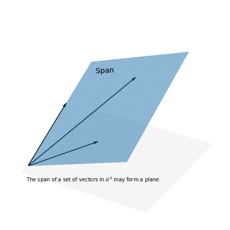
It is important to distinguish between the span of \(\{V_1, V_2, V_3, ... V_n\}\) and the actual set of vectors \(\{V_1, V_2, V_3, ... V_n\}\). The set of vectors \(\{V_1, V_2, V_3, ... V_n\}\) contains only the vectors themselves, while the span of \(\{V_1, V_2, V_3, ... V_n\}\) contains every vector that can be built as a linear combination of these vectors. If we were to visualize these objects, the set of vectors would be a collection of arrows, while the span would be a multi-dimensional collection. Again, it is easiest if we visualize an example in a two or three dimensions.
Example 1: Span in \(\mathbb{R}^4\)
We can now apply our experience in solving systems to finding linear combinations. Suppose we want to determine if \(B\) lies in the span of \(\{V_1, V_2, V_3\}\) given the following definitions.
We need to determine if there are numbers \(a_1\), \(a_2\), and \(a_3\) such that the following vector equation is true.
This vector equation is equivalent to determining if the following linear system is consistent.
We apply elimination to make a conclusion.
import numpy as np
import laguide as lag

A_augmented = np.array([[2,2,-1,4],[-1,2,-1,-2],[0,6,-1,4],[3,-4,0,2]])
A_augmented_reduced = lag.RowReduction(A_augmented)
print(A_augmented_reduced)
Pivot could not be found in column 3 .
[[ 1.   1.  -0.5  2. ]
 [ 0.   1.  -0.5  0. ]
 [ 0.   0.   1.   2. ]
 [ 0.   0.   0.   0. ]]
Since there is no pivot in the last column, the system is consistent. Recall that the key row operation in the elimination process replaces one row with the sum of itself and the multiple of another row. In other words, the rows can be replaced with a specific linear combination of rows. The row of zeros in the reduced matrix indicates that one of the four equations in the original system was in fact a linear combination of the other equations. (We don’t know for sure which equation was redundant since the rows might have been shuffled during elimination.) The remaining set of equations is triangular and we can get the solution with back substitution as before (\(a_1 = 2\), \(a_2 = 1\), \(a_3=2\)).
Example 2: Span in \(\mathbb{R}^4\)
As another example, let’s determine if the vector given as \(C\) is in the span of \(\{V_1, V_2, V_3\}\).
Again, we need to determine if the associated linear system is consistent.
B_augmented = np.array([[2,2,-1,4],[-1,2,-1,-2],[0,6,-1,4],[3,-4,0,0]])

B_reduced = lag.RowReduction(B_augmented)
print(B_reduced)
[[ 1.   1.  -0.5  2. ]
 [ 0.   1.  -0.5  0. ]
 [ 0.   0.   1.   2. ]
 [-0.  -0.  -0.   1. ]]
The pivot in the last column indicates that the system has no solution. Indeed, when we examine the system represented by the reduced matrix, we can see immediately that there are no values of \(a_1\), \(a_2\), \(a_3\) that satisfy the last equation.
Spans and inconsistent systems
The idea of spans has a direct connection to the general linear system \(AX = B\), where \(A\) is an \(m\times n\) matrix, \(X\) is in \(\mathbb{R}^n\), and \(B\) is in \(\mathbb{R}^m\). Since \(AX\) is a linear combination of the columns of \(A\), the system \(AX=B\) will have a solution if and only if \(B\) is in the span of the columns of \(A\). This is a direct result of the definitions of matrix-vector multiplication and spans. This equivalence alone doesn’t directly help us solve the system, but it does allow us to pose a more general question. For a given \(m\times n\) matrix \(A\), will the linear system \(AX=B\) have a solution for any vector \(B\) in \(\mathbb{R}^m\)?
Consider the structure of the RREF of the augmented matrix \([A|B]\) that represents an inconsistent system \(AX=B\), with \(A\) a \(4\times 4\) matrix. One possibility is the following.
The defining characteristic of an inconsistent system is that the RREF of the augmented matrix has a row with a pivot in the rightmost column. Such a row represents the equation \(0=1\). We can now realize that the system \(AX=B\) could be inconsistent if the RREF of the coefficient matrix \(A\) contains at least one row with all zero entries. This idea allows us to make a general statement about the existence of solutions. A linear system \(AX=B\) has a solution for every vector \(B\) if \(A\) has a pivot in every row
Example 3: Sets of vectors that span a space
We provide two coefficient matrices and their RREFs to demonstrate the possibilities. It should be emphasized that we are now discussing coefficient matrices, rather than the augmented matrices.
P = np.array([[1,-2,4,-2],[4,3,5,-4],[-3,-2,4,2],[-4,1,1,1]])
print(lag.FullRowReduction(P),'\n')

R = np.array([[1,1,0,-1],[1,1,0,1],[-1,-1,1,-1],[1,1,-2,0]])
print(lag.FullRowReduction(R))
[[1. 0. 0. 0.]
 [0. 1. 0. 0.]
 [0. 0. 1. 0.]
 [0. 0. 0. 1.]]

[[1. 1. 0. 0.]
 [0. 0. 1. 0.]
 [0. 0. 0. 1.]
 [0. 0. 0. 0.]]
The system \(PX=B\) has a solution for every \(B\) in \(\mathbb{R}^4\) because it has a pivot in every row. No matter which \(B\) is given, the system \(PX=B\) is always consistent. By contrast, the system \(RX=B\) will have solutions for some \(B\), but not every \(B\) in \(\mathbb{R}^4\). The span of the columns of \(P\) includes every vector in the space \(\mathbb{R}^4\). We say in this case that the columns of \(P\) span the space \(\mathbb{R}^4\).
Subspaces
It is frequently useful to consider vector subspaces, which we will simply refer to as subspaces. A subspace is a portion of a vector space with the property that any linear combination of vectors in the subspace is another vector that is also in the subspace. To put it formally, if \(V_1\) and \(V_2\) are vectors that belong to a given subspace, and \(c_1\) and \(c_2\) are any scalars, then the vector \(c_1V_1 + c_2V_2\) also belongs to the subspace.
Subspace example
The set of vectors in \(\mathbb{R}^3\) that have middle component equal to zero is a subspace of \(\mathbb{R}^3\). To understand why, we need to look at an arbitrary linear combination of two arbitrary vectors in the subspace, and verify that the linear combination is also in the subspace. If we let \(X\) and \(Y\) be the vectors with arbitrary first and third components and calculate the linear combination, we see that the linear combination also has zero as its middle component and is thus in the subspace.
Subspace non-example
The set of all solutions to the following linear system is not a subspace of \(\mathbb{R}^3\).
A_augmented = np.array([[2,1,2,0],[3,0,-1,2]])
A_augmented_reduced = lag.FullRowReduction(A_augmented)
print(A_augmented_reduced)
[[ 1.          0.         -0.33333333  0.66666667]
 [ 0.          1.          2.66666667 -1.33333333]]
In this system, \(x_3\) is a free variable. Choosing two values of \(x_3\) gives us two different solution vectors, which we label \(X_p\) and \(X_q\).
It is easy to check that the sum of these two vectors is not a solution to the system.
In fact, it is true in general that if \(A\) is an \(m\times n\) matrix, the solutions to a system \(AX=B\) do not form a subspace of \(R^m\). If \(X_p\) and \(X_q\) are two particular solutions to the system (\(AX_p=B\) and \(AX_q=B\)), their sum is not a solution since \(A(X_p + X_q) = AX_p + AX_q = B + B = 2B\).
(Note that since \(2B=B\) when \(B=0\), the set of solutions to \(AX=0\) does form a subspace. This important exception is discussed in the next section.)
Spans and subspaces
The idea of subspaces is related to that of spans since the span of any set of vectors must be a subspace. Suppose that vectors \(X\) and \(Y\) are arbitrary vectors in the span of \(\{V_1, V_2, V_3, ... V_n\}\). That is \(X = a_1V_1 + a_2V_2 + a_3V_3 + .... + a_nV_n\) and \(Y = b_1V_1 + b_2V_2 + b_3V_3 + .... + b_nV_n\) for some sets of weights \(a_1, a_2, ... a_n\) and \(b_1, b_2, ... b_n\). The arbitrary linear combination \(c_1X + c_2Y\) is also in the span of \(\{V_1, V_2, V_3, ... V_n\}\) since it is some other linear combination of these vectors.
It is also true that any subspace can be described as the span of some set of vectors. We will explore this idea in an upcoming section.
Column space
Every \(m\times n\) matrix \(A\) has associated with it four fundamental subspaces that are important in understanding the possible solutions to the linear system \(AX=B\). Here we take a look at first of these subspaces, called the column space. In future sections we will define the other three. The column space of an \(m\times n\) matrix \(A\) is defined as the span of the columns of \(A\). We think of the columns of \(A\) as vectors in \(\mathbb{R}^m\), so the column space of \(A\) forms a subspace of \(\mathbb{R}^m\). We will use the notation \(\mathcal{C}(A)\) to refer to the column space.
If \(X\) is a vector in \(\mathbb{R}^n\), then the matrix-vector product \(AX\) is a vector in \(\mathbb{R}^m\). If we recall that this product is formed by taking a linear combination of the columns of \(A\), we realize that the vector \(AX\) must be \(\mathcal{C}(A)\) by definition. An important connection here is that the linear system \(AX=B\) is consistent if and only if the vector \(B\) is in \(\mathcal{C}(A)\).
Although the concept of the column space does not actually help us solve specific systems, it does advance our ability to discuss the problem on a more abstract level. For instance, we can now fold in the definition of span, and the earlier discussion, to make a broad statement that applies to all systems. If \(A\) is an \(m\times n\) matrix, then the system \(AX=B\) is consistent for every \(B\) in \(\mathbb{R}^m\) if and only if \(\mathcal{C}(A) = \mathbb{R}^m\). Such conclusions are very important in developing further ideas which do have practical implications.
Exercises
Exercise 1: Find a linear combination of the vectors \(V_1, V_2\) and \(V_3\) which equals to the vector \(X\).
## Code solution here.
Exercise 2: Determine whether or not \(X\) lies in the span of \(\{ V_1, V_2 ,V_3\}\).
## Code solution here.
Exercise 3: Does the set \(\{ X_1, X_2 ,X_3, X_4\}\) span \(\mathbb{R}^4\)? Explain why or why not.
## Code solution here.
Exercise 4: Answer questions regarding the following vectors.
\((a)\) Determine if \(B\) is in the span of \(\{W_1, W_2, W_3\}\).
## Code solution here.
\((b)\) Determine if \(C\) is in the span of \(\{W_1, W_2, W_3\}\).
## Code solution here.
\((c)\) Find a nonzero vector in the span of \(\{W_1, W_2, W_3\}\) that has zero as its first entry.
## Code solution here.
\((d)\) How can we determine if the span of \(\{W_1, W_2, W_3\}\) equal the span of \(\{V_1, V_2\}\)?
## Code solution here.
Exercise 5: Show that the vector \(X\) lies in the span of the columns of \(A\). Also find another vector that is in the span of the columns of \(A\) and verify your answer.
Exercise 6: Consider the matrix \(R\) from Example 3. Find one vector in \(\mathbb{R}^4\) that is in the span of the columns of \(R\), and one vector in \(\mathbb{R}^4\) that is not. Demontrate with an appropriate computation.
## Code solution here.
Exercise 7: Find a vector \(V_3\) that is not in the span of \(\{ V_1, V_2\}\). Explain why the set \(\{ V_1, V_2, V_3 \}\) spans \(\mathbb{R}^3\).
## Code solution here.
Exercise 8: Explain why the system \(AX=B\) cannot be consistent for every vector \(B\) if \(A\) is a \(5\times 3\) matrix.
Exercise 9: Find the value of \(a\) for which \(\{ V_1, V_2 ,V_3\} \) does not span \(\mathbb{R}^3\).